Category Archives: ML.NET

Getting started with ML.NET in Jupyter Notebooks

For many years .NET developers have been building classic console, desktop or web applications through a stop-modify-recompile-restart cycle. In machine learning and other data-centric tasks this cycle creates so much overhead an delay that it simply doesn’t make sense. Data scientists involved in data analysis, data preparation, and model training prefer a fully interactive environment that allows mixing content, live source code, and program output in a single (web) page that gives immediate feedback when the data or the code changes.

The Jupyter ecosystem provides such an interactive environment, and there’s good news for .NET developers. The list of language kernels supported by Jupyter -including Python, R, Julia, Matlab and many others- has been extended with .NET Core.

The Jupyter Notebook app enables us today to run on-premise interactive machine learning scenarios with ML.NET using C# or F# in a web browser, without bringing software or hardware costs. In this article we try to get you started with developing and running C# machine learning scenarios in Jupyter notebooks. We’re going to assume that you already know the basics of ML.NET.

Installation

Download

There are many ways to install the environment, but you’ll always need these two ingredients:

  • the Jupiter Notebook (a Python program), and
  • dotnet interactive (formerly known as dotnet try), an version of the .NET Core runtime that allows you to run C# and F# as a scripting language.

Here’s probably the easiest way get operational – although leaner procedures may exist:

  1. Install the latest Anaconda:
    Anaconda
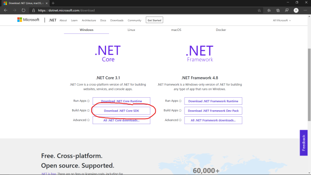
  2. Install the latest .NET Core SDK:
    NetSdk

Configure

On the command line, type the following to install dotnet interactive as a global tool:

dotnet tool install -g dotnet-try

Open the Anaconda Prompt and run the following command to register the .NET kernel in Jupyter:

dotnet try jupyter install

Validate

To verify the installation:

  • open the Anaconda3 menu from the start menu,
  • start the Jupyter Notebook app, and
  • press the ‘new’ button in the top right corner to create a new Notebook.

If .NET C# and .NET F# appear in the list of kernels, then you’re ready to go:

NetKernels

You find the most recent installation guide right here.

First steps

Fire it up

Starting a Notebook spawns a language kernel process with two clients

  • a browser with the IDE to edit and run notebooks, and
  • a terminal window displaying the logs of the associated kernel.

Here’ what to expect on your screen:

NotebookAndServer

Hello World

The browser IDE allows you to maintain a list of so-called cells. Each of these that can host documentation (markup or markdown) or source code (in the language of the kernel you selected).

Jupyter Notebooks code cells accept regular C#. Each cell can be individually ran, while the kernel keeps track of the state.

It’s safe to assume that the canonical “Hello World” would look like this:
HelloWorld1

The C# kernel hosts extra functions to control the output of cells, such as the ‘display()’ function:
HelloWorld2

Display() is more than just syntactic sugar for Console.WriteLine(). It can also render HTML, SVG, and Charts. There’s more info on this function right here.

Jupyter Notebook runs a Read-Eval-Print Loop (a.k.a. REPL). Instructions are executed, and expressions are evaluated against the current state that is maintained in and by the kernel. So instead of an instruction to print a string, you can simply type “Hello World” in a cell (without a semicolon). It will we treated as an expression:
HelloWorld3

Loading NuGet packages

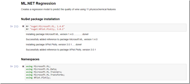
Code cells in Jupyter Notebooks can host instructions, expressions, class definitions and functions, but you can also load dll’s from NuGet packages. The #r instruction loads a NuGet package into the kernel:

NuGet


#r and using statements do not have to be written at the top of the document – you can just add them whenever you need them in the notebook.

Doing diagrams

One of the NuGet packages that you definitely want to use is XPlot, a data visualization framework written in F#. It allows you create a huge number of chart types delegating the rendering to well-known open source graphing libraries such as Plotly and Google Charts.

Here’s how easy it is to define and render a chart in a C# Jupyter Notebook:

XPlotSample

You’ll find many more examples here.

Running a Canonical Machine Learning Scenario

Over the last couple of months we have been busy creating an elaborated set of machine learning scenario’s in a UWP sample app. In the last couple of weeks we managed to migrate most of these to the Jupyter Notebook, and added some new ones.

Let’s run through one of the new samples. It predicts the quality of white wine based on 11 physicochemical characteristics. The problem is solved as a regression – in our UWP sample app we solved it as a binary and a multiclass classification.

The sample runs a representative scenario of

  • reading the raw data,
  • preparing the data,
  • training the model,
  • calculating and visualizing the quality metrics,
  • calculating and visualizing the feature contributions, and finally
  • predicting.

In this article we won’t dive into the ML.NET details. Here’s how the full scenario looks like in a Jupyter Notebook. :

Regression1

(some helpers were omitted here)Regression2

Regression3

Regression4

Regression5

Regression6

Here’s how the full web page with source and results rendering looks like.

The Jupyter Notebook provides a much more productive environment to create such a scenario than classic .NET application development does. Let’s dive into some of the reasons and take a deeper look into some Jupyter features that make the ML.NET-Jupyter combo attractive to data scientists.

Let’s focus on Data Analysis

Interactive Diagrams

Data analysis requires many types of diagrams, and Jupyter notebooks makes it easy to define and modify these.

Here’s how to import the XPlot NuGet package and render a simple interactive boxplot chart. The rendered diagram highlights the details of the element under the mouse:

InteractiveDiagram

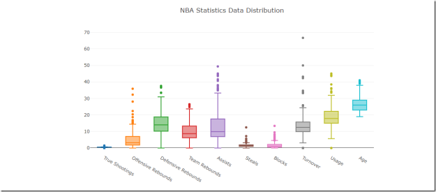
We created a more elaborated example of boxplot analysis right here. Here’s how the resulting diagram looks like:

ComplexBoxPlot

As part of Principal Component Analysis data scientists may want to draw a heat map with the correlation between different features. Here’s how easy it is to create such a chart:

HeatMap

We created a more elaborated example on the well-know Titanic data set right here. This is the resulting diagram:

TitanicHeatMap

These diagrams and many more come out-of-the-box with XPlot.

Object Formatters

Just as developers, data scientists spend most of their time debugging. They continuously need detailed feedback on the work in progress. We already encountered the new display() function that prints the value of an expression. Jupyter notebooks allow you to override the HTML that is printed for a specific class by registering an ObjectFormatter – something that sits between decorating a class with the DebuggerDisplay attribute and writing a custom debugger visualizer.

Let’s write a small –but very useful- example. Here’s how an instance of a ML.NET ConfusionMatrix is displayed by default:
ConfusionMatrix1

That’s pretty confusing, right? [Yes: pun intended!] Let’s fix this.

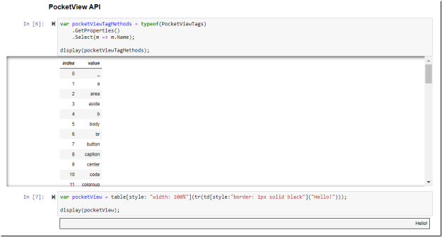
The few ObjectFormatter examples that we already encountered, were spawning IHtmlContent instances (from ASP.NET Core) that were created and styled through the so-called PocketView API – for which there is no documentation yet. Here’s how to fetch the list of HTML tags that you can create with it, and a small sample on how to apply a style to them:

var pocketViewTagMethods = typeof(PocketViewTags)
    .GetProperties()
    .Select(m => m.Name);
display(pocketViewTagMethods);

var pocketView = table[style: "width: 100%"](tr(td[style:"border: 1px solid black"]("Hello!")));
display(pocketView);

Here’s the result:

PocketView

Here’s how to register a formatter that nicely displays a table with the look-and-feel that a data analyst expects for a (binary!) confusion matrix:

Formatter.Register((df, writer) =>
{
    var rows = new List();

    var cells = new List();
    var n = df.Counts[0][0] + df.Counts[0][1] + df.Counts[1][0] + df.Counts[1][1];
    cells.Add(td[rowspan: 2, colspan: 2, style: "text-align: center; background-color: transparent"]("n = " + n));
    cells.Add(td[colspan: 2, style: "border: 1px solid black; text-align: center; padding: 24px; background-color: lightsteelblue"](b("Predicted")));
    rows.Add(tr[style: "background-color: transparent"](cells));

    cells = new List();
    cells.Add(td[style:"border: 1px solid black; padding: 24px; background-color: #E3EAF3"](b("True")));
    cells.Add(td[style:"border: 1px solid black; padding: 24px; background-color: #E3EAF3"](b("False")));
    rows.Add(tr[style: "background-color: transparent"](cells));

    cells = new List();
    cells.Add(td[rowspan: 2, style:"border: 1px solid black; text-align: center; padding: 24px;  background-color: lightsteelblue"](b("Actual")));
    cells.Add(td[style:"border: 1px solid black; text-align: center; padding: 24px; background-color: #E3EAF3"](b("True")));    
    cells.Add(td[style:"border: 1px solid black; padding: 24px"](df.Counts[0][0]));
    cells.Add(td[style:"border: 1px solid black; padding: 24px"](df.Counts[0][1]));
    rows.Add(tr[style: "background-color: transparent"](cells));

    cells = new List();
    cells.Add(td[style:"border: 1px solid black; text-align: center; padding: 24px; background-color: #E3EAF3"](b("False")));
    cells.Add(td[style:"border: 1px solid black; padding: 24px"](df.Counts[1][0]));
    cells.Add(td[style:"border: 1px solid black; padding: 24px"](df.Counts[1][1]));
    rows.Add(tr(cells));

    var t = table(
        tbody(
            rows));

    writer.Write(t);
}, "text/html");

Here’s how a confusion matrix now looks like – much more intuitive:
ConfusionMatrix2

DataFrame

It’s not always easy to prepare the data for a machine learning pipeline or a diagram, and this is where the new DataFrame API comes in. DataFrame allows you to manipulate tabular in-memory data in a spreadsheet way: you can select, add, and/or filter rows and columns, apply formulas and so on. Here’s how to pull in the NuGet package, and add a custom formatter for the base class. DataFrame is currently only in version 0.2 so you may expect some changes. You may also expect the object formatters to be embedded in future releases:


DataFrame1

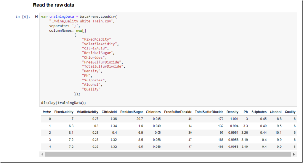
The DataFrame class knows how to read input data from a CSV:

DataFrame2

In our binary classification sample we use some of the DataFrame methods to replace the “Quality” column holding the taster’s evaluation score (a number from 1 to 10) by a “Label” column with the Boolean indicating whether the wine is good or not (i.e. the score was 6 or higher). Here’s how amazingly easy this is:

var labelCol = trainingData["Quality"].ElementwiseGreaterThanOrEqual(6);
labelCol.SetName("Label");
trainingData.Columns.Add(labelCol);
trainingData.Columns.Remove(trainingData["Quality"]);

Here’s the result (compare the last column with the one in the previous screenshot):

DataFrame3

Since there’s no documentation available yet, we had to dig into the C# source code.

DataFrame is a very promising new .NET API for tabular data manipulation, useful in machine learning and other scenarios.

Sharing is Caring

The source code of our Jupyter notebooks lives here on GitHub (if you like it then you should have put a Star on it). The easiest way to explore the code and the rendered results is via nbViewer.

We also invite you to take a look at these other ML.NET-Jupyter samples from Microsoft and from fellow MVP Alexander Slotte.

Enjoy!

Building explainable Machine Learning models with ML.NET in UWP

In this article we’ll describe how to design and build explainable machine learning models with ML.NET. We used a UWP app to host these models, and OxyPlot to create the diagrams to visualize the importance of features for a model and/or a prediction.

We will discuss the following three tasks that you can execute with the ML.NET Explainability API:

  • calculate the feature weights for a linear regression model,
  • calculate the feature contributions for a prediction, and
  • calculate Permutation Feature Importance (PFI) for a model.

The two corresponding pages it the UWP sample app look like this:

PredictionFeatureContribution

PfiCalculation

In many Machine Learning scenarios it is not only important to have a model that is accurate enough, but also to have one that is interpretable. In Health Care or Finance, models should be transparent enough to explain why they made a particular prediction. Conclusions like “You are 75% healthy” or “Your loan application was not approved” may require a better excuse than “because the computer says so”. Model explainability –knowing the importance of its features- is not only useful in justifying predictions, but also in refining the model itself – through feature selection. Investigating explainability allows you to remove features that are not significant for a model, so that you probably end up with shorter training times and less resource intensive prediction making.

The code in this article is built around the 11-features white wine quality dataset that we already covered several times in this article series. We solved it as a binary classification problem and as a multiclass classification problem for AutoML. This time we finally approach it the correct way: as a regression problem where the outcome is a (continuous) numerical value – the score– within a range. We’ll use an Stochastic Dual Coordinate Ascent regression trainer as the core of the model pipeline. Let’s first build and train that model.

Here’s the class to store the input data:

public class FeatureContributionData
{
    [LoadColumn(0)]
    public float FixedAcidity;

    [LoadColumn(1)]
    public float VolatileAcidity;

    [LoadColumn(2)]
    public float CitricAcid;

    // More features ...

    [LoadColumn(9)]
    public float Sulphates;

    [LoadColumn(10)]
    public float Alcohol;

    [LoadColumn(11), ColumnName("Label")]
    public float Label;
}

As in any ML.NET scenario we need to instantiate an MLContext:

public MLContext MLContext { get; } = new MLContext(seed: null);

Here’s the code to build and train the model. We’ll refine it later in several ways to enhance its explainability:

private IEnumerable<FeatureContributionData> _trainData;
private IDataView _transformedData;
private ITransformer _transformationModel;
private RegressionPredictionTransformer<LinearRegressionModelParameters> _regressionModel;

public List<float> BuildAndTrain(string trainingDataPath)
{
    IEstimator<ITransformer> pipeline =
        MLContext.Transforms.ReplaceMissingValues(
            outputColumnName: "FixedAcidity",
            replacementMode: MissingValueReplacingEstimator.ReplacementMode.Mean)
        .Append(MLContext.Transforms.Concatenate("Features",
            new[]
            {
                "FixedAcidity",
                "VolatileAcidity",
                "CitricAcid",
                "ResidualSugar",
                "Chlorides",
                "FreeSulfurDioxide",
                "TotalSulfurDioxide",
                "Density",
                "Ph",
                "Sulphates",
                "Alcohol"}))
        .Append(MLContext.Transforms.NormalizeMeanVariance("Features"));

    var trainData = MLContext.Data.LoadFromTextFile<FeatureContributionData>(
            path: trainingDataPath,
            separatorChar: ';',
            hasHeader: true);

    // Keep the data avalailable.
    _trainData = MLContext.Data.CreateEnumerable<FeatureContributionData>(trainData, true);

    // Cache the data view in memory. For an iterative algorithm such as SDCA this makes a huge difference.
    trainData = MLContext.Data.Cache(trainData);

    _transformationModel = pipeline.Fit(trainData);

    // Prepare the data for the algorithm.
    _transformedData = _transformationModel.Transform(trainData);

    // Choose a regression algorithm.
    var algorithm = MLContext.Regression.Trainers.Sdca();

    // Train the model and score it on the transformed data.
    _regressionModel = algorithm.Fit(_transformedData);

    // ...
}

Which features are hot, and which are not

Feature Weights in linear models

Machine Learning has several techniques for calculating how important features are in explaining/justifying the prediction. When your main algorithm is a linear classifier (e.g. linear regression) then it’s relatively easy to calculate feature contributions. The prediction is the linear combination of the features values, weighted by the model coefficients. So at model level there’s already a notion of feature contribution. In ML.NET these Weights are found in the LinearModelParameters class. This is the base class for all linear model parameter classes, like LinearRegressionModelParameters (used by SDCA) and OlsModelParameters (used by the Ordinary Least Squares trainer).

For any linear model, you can fetch the overall feature weights like this:

// Return the weights.
return _regressionModel.Model.Weights.ToList();

Here’s how the weights for the wine quality model look like in a diagram:

ModelFeatureContribution

The alcohol feature seems to dominate this particular model. Its weight is positive: a higher alcohol percentage results in a higher appreciation score. We may have just scientifically proven that alcohol is important in wine quality perception. In other news there are also at least three characteristics that could be ignored in this model – and maybe up to seven.

Feature Contribution Calculation

A second component in ML.NET’s Explainability API is a calculator that computes the list of feature contributions for a specific prediction: the FeatureContributionCalculator. Just like the overall feature weights from the previous section, the calculated feature contributions can be positive or negative. The calculator works for a large number of regression, binary classification, and ranking algorithms. The documentation page on the FeatureContributionCalculatingEstimator class contains a list of all compatible trainers. It includes

  • all linear models – because they inherently come with feature weights,
  • all Generalized Additive Models (GAM) – because their squiggly, wiggly shape functions are created by combining linear models, and
  • all tree based models – because they can calculate feature importance based on the values in the decision paths in the tree(s).

Thanks to ML.NET’s modular approach it’s easy to plug a feature contribution calculator into a model pipeline, even if the model is already trained. Here’s how we did this in the sample app.

First we extended the prediction data structure (which originally had only the Score) with an array to hold the contribution values for each feature:

public class FeatureContributionPrediction : FeatureContributionData
{
    public float Score { get; set; }

    public float[] FeatureContributions { get; set; }
}

Using the CalculateFeatureContribution() method we created and estimator, and trained it on just one input sample to become a transformer. This adds the calculation to the pipeline and the feature contributions to the output schema. The transformer was then appended to the trained model.

Here’s how that looks like in C#:

private PredictionEngine<FeatureContributionData, FeatureContributionPrediction> _predictionEngine;

public void CreatePredictionModel()
{
    // Get one row of sample data.
    var regressionData = _regressionModel.Transform(MLContext.Data.TakeRows(_transformedData, 1));

    // Define a feature contribution calculator for all the features.
    // 'Train' it on the sample row.
    var featureContributionCalculator = MLContext.Transforms
        .CalculateFeatureContribution(_regressionModel, normalize: false)
        .Fit(regressionData);

    // Create the full transformer chain.
    var scoringPipeline = _transformationModel
        .Append(_regressionModel)
        .Append(featureContributionCalculator);

    // Create the prediction engine.
    _predictionEngine = MLContext.Model.CreatePredictionEngine<FeatureContributionData, FeatureContributionPrediction>(scoringPipeline);
}

For testing the model, we didn’t dare to bother you with an input form for 11 features. Instead we added a button that randomly fetches one of the almost 4000 training samples and calculates the score and feature contributions for that sample.

Here’s the code behind this button:

public FeatureContributionPrediction GetRandomPrediction()
{
    return _predictionEngine.Predict(_trainData.ElementAt(new Random().Next(3918)));
}

Here’s how the results look like in a plot. This is an example of a linear model, so we can compare the overall model weights with the feature contributions for the specific prediction. We did not normalize the results in the feature contribution calculator configuration (the second parameter in the call) to keep these in the same range as the model weights:

PredictionFeatureContribution

Feature Contribution Calculation also works for models that don’t come with overall weights. Here’s how the results look like for a LightGBM regression trainer – one of the decision tree based algorithms:

LightGbmFeatureContribution

Check the comments in the sample app source code for its details. Also in comments, is the code for using an Ordinary Least Squares linear regression trainer. This 18th century algorithm is one is even more biased towards alcohol than our initial SDCA trainer.

For yet another example, check this official sample that adds explainability to a model covering the classic Taxi Fare Prediction scenario.

Permutation Feature Importance

The last calculator in the ML.NET Explainability API is the most computationally expensive one. It calculates the Permutation Feature Importance (PFI). Here’s how PFI calculation works:

  1. A baseline model is trained and its main quality metrics (accuracy, R squared, …) are recorded.
  2. The values of one feature are shuffled or partly replaced by random values – to undermine the relationship between the feature and the score.
  3. The modified data set is passed to the model to get new predictions and new values for the quality metrics. The result is expected to be worse than the baseline. If your model got better on random data then there was definitely something wrong with it.
  4. The feature importance is calculated as the degradation of a selected quality metric versus the one in the baseline.
  5. Steps 2, 3, and 4 are repeated for each feature so that the respective degradations can be compared: the more degradation for a feature, the more the model depends on that feature.

In ML.NET you fire up this process with a call to the PermutationFeatureImportance() method. You need to provide the model, the baseline data set, and the number of permutations – i.e. the number of feature values to replace:

// ... (same as the previous sample)

// Prepare the data for the algorithm.
var transformedData = transformationModel.Transform(trainData);

// Choose a regression algorithm.
var algorithm = MLContext.Regression.Trainers.Sdca();

// Train the model and score it on the transformed data.
var regressionModel = algorithm.Fit(transformedData);

// Calculate the PFI metrics.
var permutationMetrics = MLContext.Regression.PermutationFeatureImportance(
    regressionModel, 
    transformedData, 
    permutationCount: 50);

The call returns an array of quality metric statistics for the model type. For a regression model it’s an array of RegressionMetricStatistics instances – each holding summary statistics over multiple observations of RegressionMetrics. In the sample app we decided R Squared to be the most important quality metric. So the decrease in this value determines feature importance.

We defined a data structure to hold the result:

public class FeatureImportance
{
    public string Name { get; set; }
    public double R2Decrease { get; set; }
}

The list of feature importances is created from the result of the call and visualized in a diagram. Since we decided that R Squared is the main quality metric for our model, we used RSquared.Mean (the mean decrease in R Squared during the calculation) as the target value for feature importance:

for (int i = 0; i < permutationMetrics.Length; i++)
{
    result[i].R2Decrease = permutationMetrics[i].RSquared.Mean;
}

Here’s how the plot looks like:

PfiCalculation


We used the same regression algorithm –SDCA- as in the previous samples, so the addiction to alcohol (the feature!) should not come as a surprise anymore.

Here’s a detailed view on one of the metric statistics when debugging:

PrivateMetricsStatistics

That is an awful lot of information. Unfortunately the current API keeps most of the details private – well, you can always use Reflection. Access to more details would allow us to create more insightful diagrams like this one (source). It does not only show the mean, but also min and max values during the calculation:

importance-bike-1

For another example of explaining model predictions using Permutation Feature Importance, check this official ML.NET sample that covers house pricing.

The Source

In this article we described three components of the ML.NET Explainability API that may help you to create machine learning models that have the ability clarify their predictions. The UWP sample app hosts many more ML.NET scenario’s. It lives here on GitHub.

Enjoy!

Machine Learning with ML.NET in UWP: Automated Learning

In this article we take the ML.NET automated machine learning API for a spin to demonstrate how it can be used in a C# UWP app for discovering, training, and fine-tuning the most appropriate prediction model for a specific machine learning use case.

The Automated Machine Learning feature of ML.NET was announced at Build 2019 as a framework that automatically iterates over a set of algorithms and hyperparameters to select and create a prediction model. You only have to provide

  • the problem type (binary classification, multiclass classification, or regression),
  • the quality metric to optimize (accuracy, log loss, area under the curve, …), and
  • a dataset with training data.

The ML.NET automated machine learning functionality is exposed as

This article focuses on the automated ML API, we’ll refer to it with its nickname ‘AutoML’. In our UWP sample app we tried to implement a more or less realistic scenario for this feature. Here’s the corresponding XAML page from that app. It shows the results of a so-called experiment:

AutoML

Stating the problem

In the sample app we reused the white wine dataset from our binary classification sample. Its raw data contains the values for 11 physicochemical  characteristics -the ‘features’- of white wines together with an appreciation score from 0 to 10 – the ‘label’:

Input

We’ll rely on AutoML to build us a model that uses these physicochemical features to predict the score label. We’ll treat it as a multiclass classification problem where each distinct score value is considered a category.

Creating the DataView

AutoML requires you to provide an IDataView instance with the training data, and optionally one with test data. If the latter is not provided, it will split the training data itself. For the training data, a TextLoader on a .csv file would do the job: by default AutoML will use all non-label fields as feature, and create a pipeline with the necessary components to fill out missing values and transform everything to numeric fields. In a real world scenario you would want to programmatically perform some of these tasks yourself – overruling the defaults. That’s what we did in the sample app.

We used the LoadFromTextFile<T>() method to read the data into a new pipeline, so we needed a data structure to describe the incoming data with LoadColumn and ColumnName attributes:

public class AutomationData
{
    [LoadColumn(0), ColumnName("OriginalFixedAcidity")]
    public float FixedAcidity;

    [LoadColumn(1)]
    public float VolatileAcidity;

    [LoadColumn(2)]
    public float CitricAcid;

    [LoadColumn(3)]
    public float ResidualSugar;

    [LoadColumn(4)]
    public float Chlorides;

    [LoadColumn(5)]
    public float FreeSulfurDioxide;

    [LoadColumn(6)]
    public float TotalSulfurDioxide;

    [LoadColumn(7)]
    public float Density;

    [LoadColumn(8)]
    public float Ph;

    [LoadColumn(9)]
    public float Sulphates;

    [LoadColumn(10)]
    public float Alcohol;

    [LoadColumn(11)]
    public float Label;
}

We added a ReplaceMissingValues transformation on the FixedAcidity field to keep control over the ReplacementMode and the column names, and then removed the original column with a DropColumns transformation.

Here’s the pipeline that we used in the sample app to manipulate the raw data:

// Pipeline
IEstimator<ITransformer> pipeline =
    MLContext.Transforms.ReplaceMissingValues(
        outputColumnName: "FixedAcidity",
        inputColumnName: "OriginalFixedAcidity",
        replacementMode: MissingValueReplacingEstimator.ReplacementMode.Mean)
    .Append(MLContext.Transforms.DropColumns("OriginalFixedAcidity"));
                
    // No need to add this, it will be done automatically.
    //.Append(MLContext.Transforms.Concatenate("Features",
    //    new[]
    //    {
    //        "FixedAcidity",
    //        "VolatileAcidity",
    //        "CitricAcid",
    //        "ResidualSugar",
    //        "Chlorides",
    //        "FreeSulfurDioxide",
    //        "TotalSulfurDioxide",
    //        "Density",
    //        "Ph",
    //        "Sulphates",
    //        "Alcohol"}));

A model is created from this pipeline using the Fit() method, and the Transform() call creates the IDataView that provides the training data to the experiment:

// Training data
var trainingData = MLContext.Data.LoadFromTextFile<AutomationData>(
        path: trainingDataPath,
        separatorChar: ';',
        hasHeader: true);
ITransformer model = pipeline.Fit(trainingData);
_trainingDataView = model.Transform(trainingData);
_trainingDataView = MLContext.Data.Cache(_trainingDataView);

// Check the content on a breakpoint:
var sneakPeek = _trainingDataView.Preview();

Here’s the result of the Preview() call that allows to peek at the contents of the data view:

DataViewPreview

Keep in mind that AutoML only sees this resulting data view and has no knowledge of the pipeline that created it. It will for example struggle with data views that have duplicate column names – quite common in ML.NET pipelines.

Round 1: Algorithm Selection

Defining the experiment

In the first round of our scenario, we’ll run an AutoML experiment to find one or two candidate algorithms that we would like to explore further. Every experiment category (binary classification, multiclass classification, and regression) comes with its own ExperimentSettings class where you specify things like

  • a maximum duration for the whole experiment (AutoML will complete the test that’s running at the deadline),
  • the metric to optimize for (metrics depend on the category), and
  • the algorithms to use (by default all algorithms of the category are included in the experiment).

The experiment is then instantiated with a call to one of the Create() methods in the AutoCatalog. In the sample app we decided to optimize on Logarithmic Loss: it gives a more nuanced view into the performance then accuracy, since it punishes uncertainty. We also decided to ignore the two FastTree algorithms that are not yet 100% UWP compliant. Here’s the experiment definition:

var settings = new MulticlassExperimentSettings
{
    MaxExperimentTimeInSeconds = 18,
    OptimizingMetric = MulticlassClassificationMetric.LogLoss,
    CacheDirectory = null
};

// These two trainers yield no metrics in UWP:
settings.Trainers.Remove(MulticlassClassificationTrainer.FastTreeOva);
settings.Trainers.Remove(MulticlassClassificationTrainer.FastForestOva);

_experiment = MLContext.Auto().CreateMulticlassClassificationExperiment(settings);

Running the experiment

To execute the experiment … just call Execute() on the experiment, providing the data view and an optional progress handler to receive the trainer name and quality metrics after each individual test. The winning model is returned in the BestRun property of the experiment’s result:

var result = _experiment.Execute(
    trainData: _trainingDataView,
    labelColumnName: "Label",
    progressHandler: this);

return result.BestRun.TrainerName;

The progress handler must implement the IProgress interface which declares a Report() method that is called each time an individual test in the experiment finishes. In the sample app we let the MVVM Model implement this interface, and pass the algorithm name and the quality metrics to the MVVM ViewModel via an event. Eventually the diagram in the MVVM View -the XAML page- will be updated.

Here’s the code in the Model:

internal class AutomationModel : 
    IProgress<RunDetail<MulticlassClassificationMetrics>>
{
    // ...

    public event EventHandler<ProgressEventArgs> Progressed;

    // ...

    public void Report(RunDetail<MulticlassClassificationMetrics> value)
    {
        Progressed?.Invoke(this, new ProgressEventArgs
        {
            Model = new AutomationExperiment
            {
                Trainer = value.TrainerName,
                LogLoss = value.ValidationMetrics?.LogLoss,
                LogLossReduction = value.ValidationMetrics?.LogLossReduction,
                MicroAccuracy = value.ValidationMetrics?.MicroAccuracy,
                MacroAccuracy = value.ValidationMetrics?.MacroAccuracy
            }
        });
    }
}

The next screenshot shows the result of the algorithm selection phase in the sample app. The proposed model is not super good, but that’s mainly our own fault – the wine scoring problem is more a regression than a multiclass classification. If you consider that these models are unaware of the score order (they don’t realize that 8 is better than 7 is better than 6, etcetera – so they also not realize that a score of 4 may be appropriate if you hesitate between a 3 and a 5), then you will realize that they’re actually pretty accurate.

Here’s a graphical overview of the different models in the experiment. Notice the correlation –positive or negative- between the various quality metrics:

Round1

Some of the individual tests return really bad models. Here’s an example of an instance with a negative value for the Log Loss Reduction quality metric:

WorseThanRandom

This model performs worse than just randomly selecting a score. Make sure to run experiments long enough to eliminate such candidates.

Round 2: Parameter Sweeping

When using AutoML, we propose to first run a set of high level experiments to discover the algorithms that best suit your specific machine learning problem and, and then run a second set of experiments with a limited number of algorithms –just one or two- to fine-tune their appropriate hyperparameters. Data scientists call this parameter sweeping. For developers the source code for both sets is almost identical. In round 1 we start with all algorithms and Remove() some, and in round 2 we first Clear() the ICollection of trainers first and then Add() the few that we want to evaluate.

Here’s the full parameter sweeping code in the sample app:

var settings = new MulticlassExperimentSettings
{
    MaxExperimentTimeInSeconds = 180,
    OptimizingMetric = MulticlassClassificationMetric.LogLoss,
    CacheDirectory = null
};

settings.Trainers.Clear();
settings.Trainers.Add(MulticlassClassificationTrainer.LightGbm);

var experiment = MLContext.Auto().CreateMulticlassClassificationExperiment(settings);

var result = experiment.Execute(
    trainData: _trainingDataView,
    labelColumnName: "Label",
    progressHandler: this);

var model = result.BestRun.Model as TransformerChain<ITransformer>;

Here’s the result of parameter sweeping on the LightGbmMulti algorithm, the winner of the first round in the sample app. If you compare the diagram to the Round 1 values, you’ll observe a general improvement of the quality metrics. The orange Log Loss curve consistently shows lower values:

Round2

Not all parameter swiping experiments are equally useful. Here’s the result that compares different parameters for the LbfgsMaximumEntropy algorithm in the sample. All tests return pretty much the same (bad) model. This experiment just confirms that this is not the right algorithm for the scenario:

Round2Bis

Inspecting the Winner

After running some experiments you probably want to dive into the details of the winning model. Unfortunately this is the place where the API currently falls short: most if not all of the hyperparameters of the generated models are stored in private properties. Your options to drill down to the details are

  • open the model that you saved (it’s just a .zip file with flat texts in it), or
  • rely on Reflection.

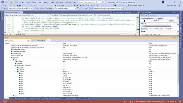
We decided to rely on the Reflection features in the Visual Studio debugger. In all multiclass classification experiments that we did, the prediction model was the last transformer in the first step of the generated pipeline. So in the sample app we assigned this to a variable to facilitate inspection via a breakpoint.

Here are the OneVersusAll parameters of the winning model. They’re the bias, the weights, splits and leaf values of the underlying RegressionTreeEnsemble for each possible score:

HyperParameters1

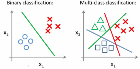
That sounds like a pretty complex structure, so let’s shed some light on it. For starters, LightGbmMulti is a so-called One-Versus-All (OVA) algorithm. OVA is a technique to solve a multiclass classification problem by a group of binary classifiers.

The following diagram illustrates using three binary classifiers to recognize squares, triangles or crosses:

one-vs-all

When the model is asked to create a prediction, it delegates the question to all three classifiers and then deducts the result. If the answers are

  • I think it’s a square,
  • I think it’s not a triangle, and
  • I think it’s not a cross,

then you can be pretty sure that it’s a square, no?

The winning model in the sample app detected 7 values for the label, so it created 7 binary classifiers. This means that not all the scores from 0 to 10 were given. [This observation made us realize that we should have treated this problem as a regression instead of as a classification.] Each of these 7 binary classifiers is a a LightGBM trainer – a gradient boosting framework that uses tree-based learning algorithms. Gradient boosting is –just like OVA- a technique that solves a problem using multiple classifiers. LightGBM builds a strong learner by combining an ensemble of weak learners. These weak learners are typically decision trees. Apparently each of the 7 classifiers in the sample app scenario hosts an ensemble of 100 trees, each with a different weight, bias, and a set of leafs and split values for each branch.

The following screenshot shows a simpler set of hyperparameters. It’s the result of a parameter sweeping round for the LbfgsMaximumEntropy algorithm, also known as multinomial logistic regression. This one is also a One-Versus-All trainer, so there are again 7 submodels. This time the models are simpler. The algorithm created a regression function for each of the score values. The parameters are the weight of each feature in that function:

HyperParameters2

At this point in time the API’s main target is to support the Command Line Tool and the Model Builder, and that’s probably why the model’s details are declared private. All of them already appear in the output of the CLI however, so we assume that full programmatic access to the models (and the source code to generate them!) is just a matter of time.

Wow!

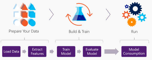
Here’s the overview of a canonical machine learning use case. The phases that are covered by AutoML are colored:

MachineLearningModel_2_3_4

To complete the scenario, all you need to do is

  • make your raw data available in an IDataView-friendly way: a .csv file or an IEnumerable (e.g. from a database query), and
  • consume the generated model in your apps, that’s just three lines of code: load the .zip file, create a prediction engine, call the prediction engine.

AutoML will do the rest. Impressive, no? There’s no excuse for not starting to embed machine learning in your .NET apps…

The Source

The sample app lives here on GitHub.

Enjoy!

Consuming an ML.NET model in UWP

In this article we’ll show step by step how to consume a Machine Learning model from ML.NET in a UWP application. In a small sample app we simulate a feedback form with a rating indicator and a text box. The app uses an existing Sentiment Analysis model to validate the assigned number of stars against the assumed (predicted) sentiment of the comments. Here’s how it looks like:

FourStarsButNegative

A typical Machine Learning scenario involves reading and manipulating training data, building and evaluating the model, and consuming the model. ML.NET supports all of these steps, as we described in our recent articles. Not all of these steps need to be hosted in the same app: you may have a central (or even external) set of applications to create the models, and another set of apps that consume these.

This article describes the latter type of apps, where the model is a ZIP file and nothing but a ZIP file.

MachineLearningModel_5

We started the project with downloading this ZIP file from the ML.NET samples on GitHub. The file contains a serialized version of the Sentiment Analysis model that was demonstrated in this Build 2019 session:

MsBuildSample

It takes an English text as input, and predicts its sentiment -positive or negative- as a probability. Data-science-wise this is a ‘binary classification by regression’ solution, but as a model consumer you don’t need to know all of this (although it definitely helps to have some basic knowledge).

Configuring the project

Here’s the solution setup. We added the ZIP file as Content in the Assets folder, and added the Microsoft.ML NuGet Package:

Configuration

This NuGet package contains most but not all of the algorithms. You may need to add more packages to bring your particular model to life (e.g. when it uses Fast Tree or Matrix Factorization).

NuGets

The model’s learning algorithm determines the output schema and the required NuGet package. The Sentiment Analysis model was built around a SdcaLogisticRegressionBinaryTrainer. Its documentation has all the necessary links:

TrainerDocumentation

Deserializing the model

In the code, we first create an MLContext as context for the other calls, and we retrieve the physical path of the model file. Then we call Model.Load() to inflate the model:

var mlContext = new MLContext(seed: null);

var appInstalledFolder = Windows.ApplicationModel.Package.Current.InstalledLocation;
var assets = await appInstalledFolder.GetFolderAsync("Assets");
var file = await assets.GetFileAsync("sentiment_model.zip");
var filePath = file.Path;

var model = mlContext.Model.Load(
    filePath: filePath,
    inputSchema: out _);

The original model file was saved without schema information, so we used the C# 7 discard (‘_’) to avoid wasting an unused local variable to the inputSchema parameter.

Defining the schema

If the schema is not persisted with the model, then you need to dive in its original source code or documentation. Here are the original input and output classes for the Sentiment Analysis model:

public class SentimentData
{
    public string SentimentText;
    [ColumnName("Label")]
    public bool Sentiment;
}

public class SentimentPrediction : SentimentData
{
    [ColumnName("PredictedLabel")]
    public bool Prediction { get; set; }
    public float Probability { get; set; }
    public float Score { get; set; }
}

Since our app will not be used to train or evaluate the model, we can get away with a simplified version of this schema. There’s no need for the TextLoader attributes or a Label column:

public class SentimentData
{
    public string SentimentText;
}

public class SentimentPrediction
{
    public bool PredictedLabel { get; set; }

    public float Probability { get; set; }

    public float Score { get; set; }

    public string SentimentAsText => PredictedLabel ? "positive" : "negative";
}

We recommend model builders to be developer friendly, and save the input schema together with the model – it’s a parameter in the Model.Save() method. This allows the consumer of the model to inspect it when loading the model. Here’s how this looks like (screenshots from another sample app):

InputSchema

When you have the input schema, you can discover or verify the output schema by creating a strongly typed IDataView and passing it to GetOutputSchema():

// Double check the output schema.
var dataView = mlContext.Data.LoadFromEnumerable<SentimentData>(new List<SentimentData>());
var outputSchema = model.GetOutputSchema(dataView.Schema);

Here’s how that looks like when debugging:

OutputSchema

Inference time

Once the input and output classes are defined, we can turn the deserialized model into a strongly typed prediction engine with a call to CreatePredictionEngine():

private PredictionEngine<SentimentData, SentimentPrediction> _engine;
_engine = mlContext.Model.CreatePredictionEngine<SentimentData, SentimentPrediction>(model);

The Predict() call takes the input (the piece of text) and runs the entire pipeline –which is a black box to the consumer- to return the result:

var result = _engine.Predict(new SentimentData { SentimentText = RatingText.Text });
ResultText.Text = $"With a score of {result.Score} " +
                  $"we are {result.Probability * 100}% " +
                  $"sure that the tone of your comment is {result.SentimentAsText}.";

The sample app compares the sentiment (positive or negative) of the text in the text box to the number of stars in the rating indicator. If these correspond, then we accept the feedback form:

FiveStarsAndPositive

When the sentiment does not correspond to the number of stars, we treat the feedback as suspicious:

OneStarButPositive

A ZIP file, an input and an output class, and five lines of code – that’s all you need for using an existing ML.NET model in your app. So far, so good.

A Word of Warning

We had two reasons to place this code in a separate app instead of in our larger UWP-ML.NET-MVVM sample app. The first reason is to show how simple and easy it is to embed and consume an ML.NET Machine Learning model in your app.

The second reason is that we needed a simple sentinel to keep an eye on the evolution of the whole “UWP-ML.NET-.NET Core-.NET Native” ecosystem. The sample app runs fine in debug mode, but in release mode it crashes. Both the creation of the MLContext and the deserialization of the model seem successful, but the creation of the prediction engine fails:

ReleaseRun

ML.NET does not fully support UWP (yet)

The UWP platform targets several devices, each with very different hardware capabilities. The fast startup for .NET applications, their small memory footprint, as well as their independence from other apps and configurations is achieved by relying on .NET Native. A release build in Visual Studio creates a native app by compiling it together with its dependencies ahead of time and stripping off al the unused code. The runtime does not come with a just-in-time compiler, so you have to be careful (i.e. you have to provide the proper runtime directives) with things like reflection and deserialization (which happen to be two popular techniques within ML.NET). On top of that, there’s the sandbox that prohibits calls to some of the Win32 API’s from within a UWP app.

When compiling the small sample app using the .NET Native Tool-Chain you’ll see that it issues warnings for some of the internal utilities projects:

ReleaseBuild

In practice, these warnings indicate that ‘some things may break at runtime’ and it is not something that we can work around as a developer.

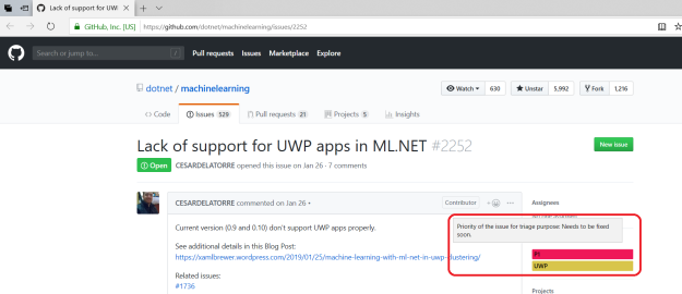
The good news is that these problems are known, an given a pretty high priority:

UwpCompatibility

The bad news is that it’s a multi team effort, involving UWP, ML.NET,.NET Core as well as .NET Native. The teams have come a long way already – a few months ago nothing even worked at debug time (that’s against the CoreCLR). But it’s extremely hard to set a deadline or a target date for full compatibility.

In one of our previous articles, we mentioned WinML as an alternative for consuming Machine Learning models. It still is, except that WinML requires the models to be persisted in the ONNX format and … export to ONNX from ML.NET is currently locked down.

In the meantime the UWP platform itself is heading to a new future with ahead-of-time compilation in .NET Core and a less restrictive sandbox. So eventually all the puzzle pieces will fall together. We just don’t know how and when. Anyway, each time that one of the components of the ecosystem is upgraded, we’ll upgrade the sample app and see what happens…

The Code

All the code for embedding and consuming an ML.NET model in a UWP app, is in the code snippets in this article. If you want to take the sample app for a spin: it lives here on GitHub.

Enjoy!

Machine Learning with ML.NET in UWP: Binary Classification

In this article we will use ML.NET to build and compare four Machine Learning Binary Classification pipelines. Each model uses another algorithm to predict the quality of wine from 11 physicochemical features. The characteristics of the prediction models are visualized using OxyPlot. All the code is in C# (“Look mom, no Python!”) and hosted in a UWP app together with some other ML.NET use cases.

Here’s how the Binary Classification sample page looks like. It displays the quality metrics of each model, and a selection of wines on which the models disagree:

SamplePageWithDisagreements

This Binary Classification sample evolved from a copy of the code and the datasets from this article on Rubik’s Code.

In the second part of this article we will focus on model evaluation and pipeline customization. We will move rapidly through the basic steps to implement a typical Machine Learning use case in ML.NET. If you want more details on each of the steps, please (re-)visit the previous articles in this series.

In the first part of this article we try to provide some relevant technical background (“Machine Learning for Developers”).

Binary Classification

Binary Classification is using a classification rule to place the elements of a given set into two groups, or to predict which group each element belongs to. In Machine Learning, Binary Classification is a part of supervised learning, which means that the classifier requires labeled (rated) samples for training and evaluation.

Math, science, decision trees, unraveling the mysteries

Binary Classification boils down to the universal problem of separating the good from the bad. It should not come as a surprise that very diverse algorithms exist, originating from very diverse domains (mathematics, probability theory, biology, operations research). Here’s a small list of Binary Classification algorithms:

  • Decision trees
  • Random forests
  • Bayesian networks
  • Support vector machines
  • Neural networks
  • Logistic regression
  • Probit model

These algorithms make different assumptions on your data and its distribution, have different performance in training and inferencing, and have different configuration options (model parameters). Fortunately there are some good resources available that help you determine the appropriate model for your Machine Learning problem, like this ‘How to choose algorithms for Azure Machine Learning Studio’. Here’s a relevant table from this article. It compares some Binary Classification models:

Algorithm Accuracy Training time Linearity Parameters Notes
Two-class classification          
logistic regression   5  
decision forest   6  
decision jungle   6 Low memory footprint
boosted decision tree   6 Large memory footprint
neural network     9 Additional customization is possible
averaged perceptron 4  
support vector machine   5 Good for large feature sets
locally deep support vector machine     8 Good for large feature sets
Bayes’ point machine   3  

If you’re more into diagrams, there’s an excellent graphical cheat sheet right here. Here’s its binary classification overview:

CheatSheet

ML.NET has implementations for most binary classification algorithms, but recommends the following trainers:

  • AveragedPerceptronTrainer
  • StochasticGradientDescentClassificationTrainer
  • LightGbmBinaryTrainer
  • FastTreeBinaryClassificationTrainer
  • SymSgdClassificationTrainer

The BinaryClassificationCatalog has more members than this. Here are all the current trainer classes:

  • AveragedPerceptronTrainer
  • BinaryClassificationGamTrainer
  • FastForestClassification
  • FastTreeBinaryClassificationTrainer
  • FieldAwareFactorizationMachineTrainer
  • LightGbmBinaryTrainer
  • LinearSvmTrainer
  • LogisticRegression
  • PriorTrainer
  • RandomTrainer (removed: https://github.com/dotnet/machinelearning/pull/2849)
  • StochasticGradientDescentClassificationTrainer
  • SymSgdClassificationTrainer

We will not compare all of these algorithms in this article, just a representative set. The choice was limited by the hosting technology: some algorithms still have some known compatibility glitches with UWP.

Here’s some background on the contestants in our comparison:

Linear Svm

Linear SVM has its roots in mathematics. A Support Vector Machine (SVM) places the training data as a p-dimensional vector (a list of p numbers) in space, and then calculates a (p-1)-dimensional hyperplane so that the examples of the separate categories are divided by a clear gap that is as wide as possible. New examples are then mapped into that same space and predicted to belong to a category based on which side of the gap they fall.

In two-dimensional space the hyperplane is just a line dividing a plane in two parts -one for each class- like in this illustration from Chris Albon:

SupportVectorClassifier

Linear SVM tries to create a hyperplane with all positive samples on one side and all negative samples on the other. Whether that works and how hard this is, depends on the data set. When the data are not linearly separable, a hinge loss function is introduced to represent the price paid for inaccurate predictions. The configuration of the model will try to minimize this function.

Linear SVM is a workhorse, simple and fast, but it may be overly simplistic for some problems. For a deeper dive into SVM, check this article.

Perceptron

The perceptron algorithm is inspired by how a brain works, and hence has its origin in biology. Perceptron can be considered as a single artificial neuron that gets an input signal for each feature, with the strength of the signal being the feature value. During training, the perceptron learns the weights for the features and stores these in its activation function. If the weighted sum of the feature values passes a threshold value, the neuron ‘fires’ and the predicted result is positive. Here’s how this looks like in an image, from “What the Hell is Perceptron”:
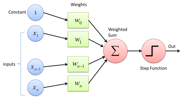
Perceptron

The learning happens one example at a time and with multiple iterations over the dataset, so you may expect long training times over larger datasets. Just like SVM, the perceptron is a linear classifier, so it will make mistakes if the data is not linearly separable. There’s an excellent deeper dive into perceptron right here.

Logistic Regression

Logistic Regression has its origin in statistics. Despite the ‘regression’ in its name (regression is predicting a continuous value) it is actually a powerful tool for two-class and multiclass classification. That is because Logistic Regression predicts a probability (“the likelihood”) – a continuous value between 0 and 1 that can easily be mapped to a class or a Boolean.

Logistic regression is not a linear classifier. ‘Logistic’ refers to a specific S-shaped curve. This logistic curve is almost linear at both extremes, and exponential in the middle. This makes it a natural fit for dividing data into groups (image from “Understanding Logistic Regression in Python”):
linear_vs_logistic_regression

Logistic Regression does not work well on data that has much outliers, or when there is high correlation between the features. Check our articles on correlation analysis and distribution analysis on how to detect and avoid these. For more details on Logistic Regression, check these course notes.

Stochastic Dual Coordinate Ascent

Stochastic Dual Coordinate Ascent (SDCA) is an algorithm for large-scale supervised learning that has its origins in mathematical programming – the science of finding the best element with regard to some criteria from a set of available alternatives. Most Machine Learning algorithms try to learn their model’s parameters by minimizing some kind of loss function, such as ordinary least squares in linear regression or the already mentioned hinge loss function. When the training set become bigger and no simple formulas exist, solving the parameters analytically (with closed-form equations) becomes economically impractical. In those cases it makes more sense to use an optimization algorithm like Coordinate Descent or Gradient Descent. Such algorithms bring you ‘close enough’ to the mathematical solution in a number of steps that each do small adjustments on the parameters. When even these calculations are too expensive, you can try reversing the problem by exploiting the duality gap (“the minimum of a curve is close enough to the maximum not on the curve”). In a nutshell, that’s what SDCA does: it iteratively reads one random (stochastic) sample from the training set and updates the model parameters, until the duality gap is sufficiently small.

Microsoft’s version of SDCA is optimized for large out-of-memory datasets and parallelism.

Decision trees

We regret that there is no Decision Tree based algorithm in our sample app. The implementations of this family of algorithms in ML.NET are currently broken for UWP.

Metrics Reloaded

Evaluating the prediction model is an essential part of any Machine Learning project. There are many metrics available to assess the quality of a model and/or compare it to another model. Most of these metrics are built around the confusion matrix which describes the performance of the model. For a two-class problem this matrix looks like this (image from Yann Dubois’ awesome Machine Learning glossary):

confusion-matrix


The confusion matrix holds the number of

  • True Positives: The cases in which the model predicted YES and the actual output was also YES,
  • True Negatives: The cases in which the model predicted NO and the actual output was NO,
  • False Positives: The cases in which the model predicted YES and the actual output was NO, and
  • False Negatives: The cases in which the model predicted NO and the actual output was YES.

Here are some common metrics for the evaluation of binary classifiers (illustrations by Chris Albon):

Accuracy

Accuracy is the ratio of the number of correct predictions to the total number of input samples.

Formula: (TP + TN) / (TP + FP + TN + FN)

Accuracy is the most common model quality metric, but it’s not always useful. For a highly unbalanced distribution and/or when the cost of making a mistake is high, accuracy is not the metric you are looking for.

Let’s say there is a one percent chance to find rare elements for car batteries somewhere in the underground, or a one percent chance of discovering some rare disease in a patient, and you want to create a prediction model for this. A model that would always return false (“computer says no”) has an accuracy of 99% in that scenario, but it would still be worthless.

Accuracy

Recall

Recall (a.k.a. Sensitivity) is the fraction of positive observations that have been correctly predicted.

Formula: TP / (TP + FN)

If missing a positive example is important/expensive, you should focus on maximizing recall.

Recall

Specificity

Specificity is the recall for the negatives (the ability to find true negatives).

Formula: TN / (TN + FP)

Precision

Precision is fraction of positive predictions that were actually positive.

Formula: TP / (TP + FP)

If false positives are expensive, maximize precision.

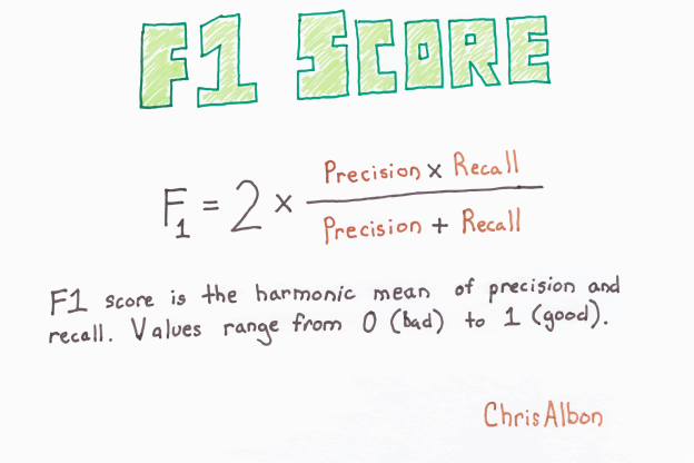
F1 Score

F1 score is the harmonic mean between precision and recall. If one of these two values decreases dramatically, the F1 score also does. F1 score reaches its best value at 1 (perfect precision and recall) and worst at 0.

Formula: 2 * (Precision * Recall) / (Precision + Recall)

F1 score tells you how precise your classifier is (how many instances it classifies correctly) as well as how robust it is (it does not miss significant groups of instances).
F1Score

Area under the ROC curve

Area Under Curve (AUC) is one of the most widely used metrics for the evaluation of binary classifiers. AUC is the probability that the classifier will rank a randomly chosen positive example higher than a randomly chosen negative example. The referenced curve is called Receiving Operating Characteristic (ROC) and plots the True Positive Rate (TP / (TP + FN)) against the False Positive Rate (FP / (FP + TN)) for all probability thresholds.

AreaUnderTheCurve

Plotting the curve is an expensive operation, but calculating the area under it is not. AUC measures the entire two-dimensional area underneath the entire ROC curve from (0,0) to (1,1). The result is a value between 0.5 (which means that your model behaves like random classifier) and 1 (too good to be true, you’re probably overfitting).

More Metrics

There are more metrics to evaluate and compare binary classifiers, especially the classifiers that return a probability: Logarithmic Loss and Cross-Entropy and more. Not all algorithms in our sample app are in this category, so we decided to ignore these metrics for the moment.

Now is the time to dive into the code.

Battle of the Binary Stars

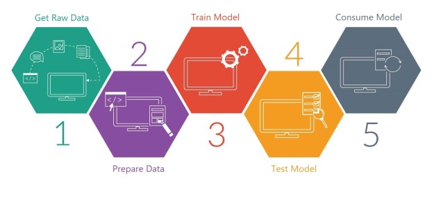
We’re in a traditional Machine Learning use case with reading and preparing the data, training and evaluating the model, and finally using the model for predicting:
MachineLearningModel

Getting the Raw Data

Here’s how the training and testing data sets look like. They list 11 physicochemical and sensory characteristics of Portuguese Vinho Verde white wine, together with a quality score on a scale of 10:

WineQualityDataSet

Here’s the corresponding input structure. We decorated the fields with the LoadColumn attribute to facilitate reading the file with one of the built-in ML.NET text readers:

public class BinaryClassificationData
{
    [LoadColumn(0)]
    public float FixedAcidity;

    [LoadColumn(1)]
    public float VolatileAcidity;

    [LoadColumn(2)]
    public float CitricAcid;

    [LoadColumn(3)]
    public float ResidualSugar;

    [LoadColumn(4)]
    public float Chlorides;

    [LoadColumn(5)]
    public float FreeSulfurDioxide;

    [LoadColumn(6)]
    public float TotalSulfurDioxide;

    [LoadColumn(7)]
    public float Density;

    [LoadColumn(8)]
    public float Ph;

    [LoadColumn(9)]
    public float Sulphates;

    [LoadColumn(10)]
    public float Alcohol;

    [LoadColumn(11), ColumnName("Label")]
    public float Label;
}

The models will predict the quality of the wine as a Boolean – good or bad. Here’s how the output structure looks like:

public class BinaryClassificationPrediction
{
    [ColumnName("PredictedLabel")]
    public bool PredictedLabel;

    public int LabelAsNumber => PredictedLabel ? 1 : 0;
}

The file is read with LoadFromTextFile() and stored in memory with Cache(). The latter will improve the training speed for the online learners -the ones that iteratively read a sample- such as SDCA:

var trainData = MLContext.Data.LoadFromTextFile<BinaryClassificationData>(
        path: trainingDataPath,
        separatorChar: ';',
        hasHeader: true);

trainData = MLContext.Data.Cache(trainData);

When this code runs, the training data becomes available as an IDataView.

Preparing the data

In ML.NET, the model is defined by a pipeline of components that each apply transformations to the data. Some transformations make the data more representative and compatible with the classifier, other transformations skip the training data with missing or out-of-range values (outliers).

Here are the pipeline steps for our sample:

  • fill out missing values for Fixed Acidity,
  • translate the numeric quality score to a Boolean,
  • create a vector with all feature values, and
  • add one of the binary classifiers.

Here’s how that pipeline looks like in C#:

public PredictionModel<BinaryClassificationData, BinaryClassificationPrediction> BuildAndTrain(
    string trainingDataPath,
    IEstimator<ITransformer> algorithm)
{
    IEstimator<ITransformer> pipeline =
        MLContext.Transforms.ReplaceMissingValues(
            outputColumnName: "FixedAcidity",
            replacementMode: MissingValueReplacingEstimator.ReplacementMode.Mean)
        .Append(MLContext.FloatToBoolLabelNormalizer())
        .Append(MLContext.Transforms.Concatenate("Features",
            new[]
            {
                "FixedAcidity",
                "VolatileAcidity",
                "CitricAcid",
                "ResidualSugar",
                "Chlorides",
                "FreeSulfurDioxide",
                "TotalSulfurDioxide",
                "Density",
                "Ph",
                "Sulphates",
                "Alcohol"}))
        .Append(algorithm);

    // ...

}

Let’s get into the details of some of the preparation steps.

Dealing with missing values

Input data that has missing values for one or more features can ruin the training of your prediction model. ML.NET comes with some useful transforms to deal with this:

Building a Custom Data Transformation Component

The FloatToBoolNormalizer in the previous code snippet is a transformation component that we wrote ourselves. It transforms the numeric quality column from the dataset into a Boolean, without relying on hard-coded thresholds. Boolean is the required data type for the binary classifier’s Label column.

The custom component is a mini pipeline on its own: an IEstimator<ITransformer>. We start with dividing all the values into two bins or buckets (feel free to pronounce it as “bouquets”) of the same size, using NormalizeBinning() from the NormalizationCatalog. After this first transformation the Label column now holds 0 or 1, where the algorithm still expects a Boolean.

To transform the 0-or-1 to a Boolean, we created a CustomMappingFactory with some helper input and output classes, and the appropriate CustomMappingFactory attribute. It is appended with CustomMapping() to the mini pipeline.

The whole component is made reusable in multiple ML.NET pipelines by exposing it as an extension method to MLContext:

public static class MLContextExtensions
{
    /// <summary>
    /// Divides the numeric Label in two 'buckets' and transforms it to a Boolean.
    /// </summary>
    public static IEstimator<ITransformer> FloatToBoolLabelNormalizer(this MLContext mLContext)
    {
        var normalizer = mLContext.Transforms.NormalizeBinning(
            outputColumnName: "Label", maximumBinCount: 2);

        return normalizer.Append(mLContext.Transforms.CustomMapping(new MapFloatToBool().GetMapping(), "MapFloatToBool"));
    }

    private class LabelInput
    {
        public float Label { get; set; }
    }

    private class LabelOutput
    {
        public bool Label { get; set; }

        public static LabelOutput True = new LabelOutput() { Label = true };
        public static LabelOutput False = new LabelOutput() { Label = false };
    }

    [CustomMappingFactoryAttribute("MapFloatToBool")]
    private class MapFloatToBool : CustomMappingFactory<LabelInput, LabelOutput>
    {
        public override Action<LabelInput, LabelOutput> GetMapping()
        {
            return (input, output) =>
            {
                if (input.Label > 0)
                    output.Label = true;
                else
                    output.Label = false;
            };
        }
    }
}

For another example and more details, check the excellent ML.NET Cook Book.

Training the Models

We now have a training data set in memory, and a pipeline with all necessary transformation components. All we need to do to create the model is call Fit() and turn it into a PredictionEngine:

ITransformer model = pipeline.Fit(trainData);
return new PredictionModel<BinaryClassificationData, BinaryClassificationPrediction>(
	MLContext, 
	model);

The PredictionModel is a reconstruction of a class that disappeared from the API when we we building the sample app. We have kept it in the code as a little helper to keep the algorithm and its prediction engine together:

public PredictionModel(MLContext mlContext, ITransformer transformer)
{
    Transformer = transformer;
    Engine = mlContext.Model.CreatePredictionEngine<TSrc, TDst>(Transformer);
}

All what’s left to build the models is instantiate each of the four algorithms that we’re going to compare:

Here are the private fields to hold all of these:

private PredictionModel<BinaryClassificationData, BinaryClassificationPrediction> _perceptronBinaryModel;
private PredictionModel<BinaryClassificationData, BinaryClassificationPrediction> _linearSvmModel;
private PredictionModel<BinaryClassificationData, BinaryClassificationPrediction> _logisticRegressionModel;
private PredictionModel<BinaryClassificationData, BinaryClassificationPrediction> _sdcabModel;

And these are the calls to build and train all four models:

_perceptronBinaryModel = await ViewModel.BuildAndTrain(trainingDataLocation, ViewModel.MLContext.BinaryClassification.Trainers.AveragedPerceptron());
_linearSvmModel = await ViewModel.BuildAndTrain(trainingDataLocation, ViewModel.MLContext.BinaryClassification.Trainers.LinearSvm());
_logisticRegressionModel = await ViewModel.BuildAndTrain(trainingDataLocation, ViewModel.MLContext.BinaryClassification.Trainers.LbfgsLogisticRegression());
_sdcabModel = await ViewModel.BuildAndTrain(trainingDataLocation, ViewModel.MLContext.BinaryClassification.Trainers.SdcaLogisticRegression());

We confess that this code is implemented in the MVVM View and we probably deserve a Walk of Atonement for this (“shame … shame … shame”). We just did not know upfront which and how many of the algorithms would work in a UWP context, hence the exploratory code patterns.

Testing the Models

Binary classifiers fall into two categories (pun intended): the ones that return a category class, and the ones that return a probability. In ML.NET both types have another class for their metrics: BinaryClassificationMetrics versus CalibratedBinaryClassificationMetrics. Fortunately there is an inheritance relationship between these two: the calibrated class extends the list of standard binary metrics (such as Accuracy, F1Score, the whole ConfusionMatrix, and the AreaUnderRocCurve) with the probability-related ones (such as LogLoss and Entropy).

The ML.NET API confusingly forces two different calls to trigger the evaluation: Evaluate() versus EvaluateNonCalibrated(). Here are the wrapper methods in the sample app that load and prepare the test data set, generate predictions with Transform(), compare the predicted with the actual results, and finally return the metrics:

public CalibratedBinaryClassificationMetrics Evaluate(
    PredictionModel<BinaryClassificationData, BinaryClassificationPrediction> model,
    string testDataLocation)
{
    var testData = MLContext.Data.LoadFromTextFile<BinaryClassificationData>(
        path: testDataLocation,
        separatorChar: ';',
        hasHeader: true);

    var scoredData = model.Transformer.Transform(testData);
    return MLContext.BinaryClassification.Evaluate(scoredData);
}

public BinaryClassificationMetrics EvaluateNonCalibrated(
    PredictionModel<BinaryClassificationData, BinaryClassificationPrediction> model,
    string testDataLocation)
{
    var testData = MLContext.Data.LoadFromTextFile<BinaryClassificationData>(
        path: testDataLocation,
        separatorChar: ';',
        hasHeader: true);

    var scoredData = model.Transformer.Transform(testData);
    return MLContext.BinaryClassification.EvaluateNonCalibrated(scoredData);
}

Here’s the call in the View that fetches these metrics:

BinaryClassificationMetrics metrics = await ViewModel.EvaluateNonCalibrated(_perceptronBinaryModel, _testDataPath);

Again, there are some violations of the MVVM pattern here, but we did not know which and how many of these metrics would end up in the diagram.

Here’s how the metrics are visualized with a bar chart in the sample app:

SamplePage

The lack of quality in the two models on the left is clearly noticeable. The good wines do not seem to be linearly separable from the bad wines. It seems that logistic regression is the way to go in this particular scenario. The dataset is also not big enough to justify SDCA, the last algorithm is not better than the third, but is clearly a lot slower.

Saving the Models

The ML.NET API could not be more straightforward: use Model.Save() to … save the model:

public void Save(
    PredictionModel<BinaryClassificationData, BinaryClassificationPrediction> model,
    string modelName)
{
    var storageFolder = ApplicationData.Current.LocalFolder;
    string modelPath = Path.Combine(storageFolder.Path, modelName);

    MLContext.Model.Save(
        model: model.Transformer,
        inputSchema: null,
        filePath: modelPath);
}

Consuming the Models

We assume that in most cases you’ll be interested at runtime in assessing the quality of just a limited number of wines, so we built the prediction method around PredictionEngine.Predict() – the call to generate a single prediction:

public IEnumerable<BinaryClassificationPrediction> Predict(
    PredictionModel<BinaryClassificationData, BinaryClassificationPrediction> model,
    IEnumerable<BinaryClassificationData> data)
{
    foreach (BinaryClassificationData datum in data)
        yield return model.Engine.Predict(datum);
}

The sample app uses this method to get predictions from each of the 4 models for the first 50 wines in the test data set:

var testDataLocation = await MlDotNet.FilePath(@"ms-appx:///Data/winequality_white_test.csv");
var tests = await ViewModel.GetSample(testDataLocation);
var size = 50;
var data = tests.ToList().Take(size);

var perceptronPrediction = (await ViewModel.Predict(_perceptronBinaryModel, data)).ToList();
var linearSvmPrediction = (await ViewModel.Predict(_linearSvmModel, data)).ToList();
var logisticRegressionPrediction = (await ViewModel.Predict(_logisticRegressionModel, data)).ToList();
var sdcabPrediction = (await ViewModel.Predict(_sdcabModel, data)).ToList();

This code gets called when you click the ‘View Disagreements’ button. Observe that the models –even from the same family (linear or logistic)- disagree on quite some samples.

The table in the center of the page lists the differences:

SamplePageWithDisagreements

It is clear that the linear models are the drama queens in this setup. They’re too easily overoptimistic or overpessimistic on the quality of the wines.

All the code and more

The UWP sample app lives here on GitHub. It hosts a lot more ML.NET scenarios than what we covered in this article. Look at the code, play with the code. If it sparks joy, please return the favor and give the repo a star!

Enjoy!

Machine Learning with ML.NET in UWP: Field-Aware Factorization Machine

In this article we demonstrate how to use a Field-Aware Factorization Machine to recommend hotels on the Las Vegas Strip, based on the traveler type (solo, family, business, …) and the season. We’ll use ML.NET for the Machine Learning stuff, OxyPlot for visualization, and a UWP app to host it all. This is how the sample page looks like:

FfmRecommendation

This page looks pretty much like the one in our previous article on recommendation in Machine Learning. That article also recommended hotels – but since we were using Matrix Factorization we could only use one feature to base the recommendation on (i.c. traveler type). In the previous article, the prediction model was defined by preparing the two feature columns (TravelerType and Hotel) and passing these to a recommendation algorithm, like this:

var pipeline = _mlContext.Transforms.Conversion.MapValueToKey("Hotel")
                .Append(_mlContext.Transforms.Conversion.MapValueToKey("TravelerType"))
                .Append(_mlContext.Recommendation().Trainers.MatrixFactorization(
                                    labelColumnName: "Label",
                                    matrixColumnIndexColumnName: "Hotel",
                                    matrixRowIndexColumnName: "TravelerType"))
                .Append(_mlContext.Transforms.Conversion.MapKeyToValue("Hotel"))
                .Append(_mlContext.Transforms.Conversion.MapKeyToValue("TravelerType"));

The corresponding pipeline in this article would look very similar:

var pipeline = _mlContext.Transforms.Categorical.OneHotEncoding("TravelerTypeOneHot", "TravelerType")
                .Append(_mlContext.Transforms.Categorical.OneHotEncoding("HotelOneHot", "Hotel"))
                .Append(_mlContext.Transforms.Concatenate("Features", "TravelerTypeOneHot", "HotelOneHot"))
                .Append(_mlContext.BinaryClassification.Trainers.FieldAwareFactorizationMachine(new string[] { "Features" }));

The advantage of a Field-Aware Factorization Machine over Matrix Factorization is that you’re not limited to two features. This allows you to provide much better recommendations. Hotels could be recommended on a combination of traveler type, season, country of origin, etc.

Field-Aware Factorization in Machine Learning

A Field-Aware Factorization Machine (FFM) is a recommendation algorithm that is specialized in deriving knowledge from large and sparse datasets. It recognizes feature conjunctions in feature vectors. This is particularly useful in Click-Through Rate prediction (CTR). Check this article for an introduction and a comparison to other algorithms.

The FFM algorithm takes a vector of numerical features as input. When we’re dealing with categorical data (countries, months, traveler types, …) we need to transform these into numbers. In the context of FFM the right approach is to use One-Hot Encoding, which boils down to pivoting feature values into separate columns. There’s an excellent beginners guide to one-hot encoding right here, but this illustration from Chris Albon’s Machine Learning Flashcards says it all:


One-Hot_Encoding

The one-hot encoding transformation extends the schema with a lot of new features, sparsely filled. That exactly how FFM likes it…

Field-Aware Factorization in ML.NET

With the FieldAwareFactorizationMachineTrainer and the OneHotEncodingTransformer, ML.NET has all the ingredients to implement a Field-Aware Factorization Machine scenario.

Let’s write some code

Here’s how a typical Machine Learning use case looks like:

MachineLearningModel

Raw data is collected, then cleaned up, completed, and transformed to fit the algorithm. Part of the data is used to train the model, another part is used to evaluate it. When the model passed all tests, it is persisted for consumption.

The sample app uses a light-weight MVVM architecture. The beef of the ML.NET manipulation is in this Model class.

Getting the Raw Data

The raw data in the sample app comes from a comma-separated flat file with Trip Advisor reviews from 2015 for hotels on the Las Vegas Strip:

RecommendationDataSet

Preparing the Data

While we read the data, we already start the preparation. FFM is a binary classification algorithm, so we need to transform the rating (0-5) to a Boolean value (“recommended or not”). Here’s the input structure:

public class FfmRecommendationData
{
    public bool Label;

    public string TravelerType;

    public string Season;

    public string Hotel;
}

The predicted label will also be a Boolean, and the algorithm also provides the corresponding probability. Here’s the model’s output structure:

public class FfmRecommendationPrediction
{
    public bool PredictedLabel;

    public float Probability;

    public string TravelerType;

    public string Season;

    public string Hotel;
}

Before we read all the data in an IDataView, we need to create a MLContext instance:

private MLContext _mlContext = new MLContext(seed: null);

While we read the data, we transform the score (0 to 5) into a Boolean by comparing it to a threshold value. We used 3 as the threshold, since the general ratings in the dataset are pretty high – which is probably why these were allowed to make public.

With the LoadFromEnumerable() method we transform it into an IDataView:

private IDataView _allData;
private ITransformer _model;

public IEnumerable<FfmRecommendationData> Load(string trainingDataPath)
{
    // Populating an IDataView from an IEnumerable.
    var data = File.ReadAllLines(trainingDataPath)
        .Skip(1)
        .Select(x => x.Split(';'))
        .Select(x => new FfmRecommendationData
        {
            Label = double.Parse(x[4]) > _ratingThreshold,
            Season = x[5],
            TravelerType = x[6],
            Hotel = x[13]
        });

    _allData = _mlContext.Data.LoadFromEnumerable(data);

    // Just 'return data;' would also do the trick...
    return _mlContext.Data.CreateEnumerable<FfmRecommendationData>(_allData, reuseRowObject: false);
}

For the next step in preparing the data we will rely on some ML.NET transformations. First we apply a OneHotEncoding transformation to all the features, to transform the categorical data into numbers. Then all features are combined into a vector with a call to Concatenate(). The model building pipeline is then completed with a FieldAwareFactorizationMachine:

var pipeline = _mlContext.Transforms.Categorical.OneHotEncoding("TravelerTypeOneHot", "TravelerType")
    .Append(_mlContext.Transforms.Categorical.OneHotEncoding("SeasonOneHot", "Season"))
    .Append(_mlContext.Transforms.Categorical.OneHotEncoding("HotelOneHot", "Hotel"))
    .Append(_mlContext.Transforms.Concatenate("Features", "TravelerTypeOneHot", "SeasonOneHot", "HotelOneHot"))
    .Append(_mlContext.BinaryClassification.Trainers.FieldAwareFactorizationMachine(new string[] { "Features" }));

Training the Model

To train the model, we send 450 randomly chosen rows from the dataset to it. The rows are selected with some methods from the DataOperationsCatalog: first we rearrange the dataset with ShuffleRows(), then we pick some rows with TakeRows():

var trainingData = _mlContext.Data.ShuffleRows(_allData);
trainingData = _mlContext.Data.TakeRows(trainingData, 450);

After training the model, we’ll create a strongly typed PredictionEngine from it, for individual recommendations. So we declared a field to host this:

private PredictionEngine<FfmRecommendationData, FfmRecommendationPrediction> _predictionEngine;

The model is created and trained with a call to Fit(), and then we create the prediction engine from it with CreatePredictionEngine():

_model = pipeline.Fit(trainingData);
_predictionEngine = _mlContext.Model.CreatePredictionEngine<FfmRecommendationData, FfmRecommendationPrediction>(_model);

Testing the Model

To test the model we send another 100 random rows from the dataset to it and call the Transform() to generate the predictions. A call to the Evaluate() method in the BinaryClassificationCatalog will compare the predicted labels to the original ones:

public CalibratedBinaryClassificationMetrics Evaluate(string testDataPath)
{
    var testData = _mlContext.Data.ShuffleRows(_allData);
    testData = _mlContext.Data.TakeRows(testData, 100);

    var scoredData = _model.Transform(testData);
    var metrics = _mlContext.BinaryClassification.Evaluate(
        data: scoredData, 
        labelColumnName: "Label", 
        scoreColumnName: "Probability", 
        predictedLabelColumnName: "PredictedLabel");

    // Place a breakpoint here to inspect the quality metrics.
    return metrics;
}

The result of the evaluation is an instance of CalibratedBinaryClassificationMetrics with useful statistics such as accuracy, entropy, recall, and F1-score:

CalibratedMetrics

Persisting the Model

When you’re happy with the model’s quality, then you can serialize and persist it for later use with a call to the Save() method from the ModelOperationsCatalog:

public void Save(string modelName)
{
    var storageFolder = ApplicationData.Current.LocalFolder;
    string modelPath = Path.Combine(storageFolder.Path, modelName);

    _mlContext.Model.Save(_model, inputSchema: null, filePath: modelPath);
}

Consuming the Model

There are two ways to consume the model. With a call to Transform() you can generate predictions or recommendations for a group of input records. The resulting IDataView can be transformed to a list of prediction records with CreateEnumerable():

public IEnumerable<FfmRecommendationPrediction> Predict(IEnumerable<FfmRecommendationData> recommendationData)
{
    // Group prediction
    var data = _mlContext.Data.LoadFromEnumerable(recommendationData);
    var predictions = _model.Transform(data);
    return _mlContext.Data.CreateEnumerable<FfmRecommendationPrediction>(predictions, reuseRowObject: false);
}

The strongly typed PredictionEngine that we created after training the model, can be used for single recommendation. Its Predict() method runs the prediction pipeline for a single input record:

public FfmRecommendationPrediction Predict(FfmRecommendationData recommendationData)
{
    // Single prediction
    return _predictionEngine.Predict(recommendationData);
}

When the predicted label is false, the model does not recommend the hotel/travelertype/season combination. In that case we reverse the displayed probability (the score) so that its values become a range from –1 (strongly discouraged) to +1 (strongly recommended). This is done in the MVVM View (the code-behind in the page):

var result = await ViewModel.Predict(recommendationData);
if (!result.PredictedLabel)
{
    // Bring to a range from -1 (highly discouraged) to +1 (highly recommended).
    result.Probability = -result.Probability;
}


The Model in Action

Here’s the FFM Recommendation page from the sample app again:

FfmRecommendation

When the model is ready for operation, the combo boxes are populated and unlocked. When you change the traveler type or the season, a group prediction is done for all the hotels in the data set. Its result is displayed on the left in a horizontal bar chart. We’ll not diving into its details, since it’s basically the same diagram as the one in the previous article (we’re just displaying the probability (-1 to +1) instead of the predicted rating (0 to 5).

When you select a hotel in the combo box in the bottom left corner, a single prediction is made, and the result is displayed next to it. The diagram for the group predictions only displays recommended hotels, but in the single prediction you can pick your own hotel. That’s why we decided to display a negative probability for negative advice.

If you want to run this scenario yourself, feel free to download the sample app. Its source lives here on GitHub.

Enjoy!

Machine Learning with ML.NET in UWP: Recommendation

In this article we describe how to define, train, evaluate, persist, and use a ML.NET Recommendation model in a UWP app. The blog post is part of a series on implementing different Machine Learning scenarios with .NET Open Source frameworks and components such as

All articles in the series are supported by the same UWP sample app that lives here on GitHub. Since the previous article was published, this sample app was upgraded to the latest prereleases of ML.NET thanks to Pull Requests from the Microsoft ML.NET Team itself (thanks Eric!). This means that the syntax in the code snippets is quite different from the previous articles, but much closer to the imminent official release.

Here’s how the Recommendation page in the sample app looks like:

Recommendation

It builds a model to generate recommendations for hotels on the Las Vegas Strip for a selected traveler type (single, family, business, …):

  • when you select a traveler type in the combo box, the top 10 recommended hotels appear in the diagram, and
  • when you select a hotel in the second combo box, a predicted rating will appear next to it.

Recommendation in Machine Learning

Machine Learning recommender systems are highly popular in e-commerce and social networks. They’re used for recommending books, TV series, music, events, products, friends, dating profiles, and a lot more.

There are two approaches for generating recommendations:

  • Content Based Filtering recommends items to a user that are similar to previously highly rated items by the same user. The advantage of this is transparency (the model can explain why it recommends the item). Unfortunately this approach does not scale well with large data.
  • Collaborative Based Filtering will recommend the items to a user that were highly rated by other -but similar- users. In most real world scenarios not every user has rated every item, so the base data can be very sparse. This makes the approach unsuitable in some scenarios.

Matrix Factorization in Machine Learning

Matrix Factorization is a common technique to solve the sparsity problem with Collaborative Base Filtering that we just mentioned. In a nutshell its goal is to mass-predict the missing ratings. Matrix Factorization is entirely based on linear algebra which is something that your CPUs, GPUs, and/or AI Accelerators are pretty good at. If you want to dive into the mathematical details, allow me to recommend (pun intended) the article with the very appropriate name A Gentle Introduction to Matrix Factorization for Machine Learning.

Major advantages of this algorithm are that it scales very well with large data and it is very fast. You don’t have take my word for it, but there must me a reason why Amazon and Netflix are relying on it. The algorithm has the disadvantage that it cannot always easy explain why it recommends an item. You must have stumbled upon recommendations like this before:

netflix

Before we dive into the code, allow us to clarify something: Matrix Factorization does NOT answer the question “What items would you recommend for this user?”. Instead it solves the “Here’s a list of products and a (list of) user(s), please predict their ratings” problem. So when you use it in your apps, there is some preprocessing (selecting the products to evaluate) and some postprocessing (filtering relevant recommendation) to do. Basically the algorithm always has to deal with too much data. Don’t worry about that: Matrix Factorization is a real Weapon of Mass Prediction

Matrix Factorization in ML.NET

For Matrix Factorization in ML.NET you’ll need the MatrixFactorizationTrainer class. It comes in a separate NuGet package (Microsoft.ML.Recommender):

RecommenderNuGet

Model Input and Output

For training and testing the model, we’ll use a 2015 dataset with 510 Las Vegal hotel ratings from TripAdvisor. Here’s how it looks like:

RecommendationDataSet

Matrix Factorization predicts the rating (“Label”) between only two fields (“Features”) . If you have to deal with more fields, then you’ll need the FieldAwareFactorizationMachine instead.

In the sample app we choose TravelerType and Hotel as features to respectively play the roles of ‘similar user’ and ‘recommended item’. The Score column contains the rating and will play the role of ‘label’ (the thing to predict). Since the prediction engine’s output column is also called Score, we renamed it to Label for the input.

Here’s the structure of input samples that we will feed the model with:

public class RecommendationData
{
    public float Label;

    public string TravelerType;

    public string Hotel;
}

The prediction looks like this:

public class RecommendationPrediction
{
    public float Score;

    public string TravelerType;

    public string Hotel;
}

Observe the lack of LoadColumn and ColumnName attributes on top of the fields – we had these in all the previous posts in this article series. We don’t need the attributes here because we’re not using a TextLoader to read the training and testing data sets. Instead we’ll create our IDataView with a call to the LoadFromEnumerable() method. This same method allows you to populate the model with records from a database:

private IDataView trainingData;

public IEnumerable<RecommendationData> Load(string trainingDataPath)
{
    var data = File.ReadAllLines(trainingDataPath)
        .Skip(1)
        .Select(x => x.Split(';'))
        .Select(x => new RecommendationData
        {
            Label = uint.Parse(x[4]),
            TravelerType = x[6],
            Hotel = x[13]
        })
        .OrderBy(x => (x.GetHashCode())) // Cheap Randomization.
        .Take(400);

    // Populating an IDataView from an IEnumerable.
    trainingData = _mlContext.Data.LoadFromEnumerable(data);

    // Keep DataView in memory.
    trainingData = _mlContext.Data.Cache(trainingData);

    // Populating an IEnumerable from an IDataView.
    return _mlContext.Data.CreateEnumerable<RecommendationData>(trainingData, reuseRowObject: false);
}

Part of the data set will be used for training, and another for evaluating the model. Since the original data set is sorted on Hotel name, we applied cheap randomization logic to the rows by sorting them on their GetHashCode() value.

The Cache() method keeps the selected columns (in our case: all columns) in memory after they’re accessed for the first time. For iterative algorithms this really is a time saver – at least if the data fits into memory.

Defining and Building the Model

The recommendation model is an ITransformer that is created from an EstimatorChain with a MatrixFactorization at its heart. You have to specify the label (labelColumn) and the two features (matrixRowIndexColumnName and matrixColumnIndexColumnName) and some options to fine tune the algorithm. Before sending the feature values to the transformer, they’re added to a dictionary with MapValueToKey(). The reverse function of that is MapKeyToValue(). It ensures that the original values are returned with the predicted score.

Here’s the whole pipeline:

private ITransformer _model;

public void Build()
{
    var pipeline = _mlContext.Transforms.Conversion.MapValueToKey("Hotel")
                    .Append(_mlContext.Transforms.Conversion.MapValueToKey("TravelerType"))
                    .Append(_mlContext.Recommendation().Trainers.MatrixFactorization(
                                        labelColumn: DefaultColumnNames.Label,
                                        matrixColumnIndexColumnName: "Hotel",
                                        matrixRowIndexColumnName: "TravelerType",
                                        // Optional fine tuning:
                                        numberOfIterations: 20,
                                        approximationRank: 8,
                                        learningRate: 0.4))
                    .Append(_mlContext.Transforms.Conversion.MapKeyToValue("Hotel"))
                    .Append(_mlContext.Transforms.Conversion.MapKeyToValue("TravelerType"));

    // Place a breakpoint here to peek the training data.
    var preview = pipeline.Preview(trainingData, maxRows: 10);

    _model = pipeline.Fit(trainingData);
}

The extremely useful Preview() method was recently added to the API. It allows you to inspect the content and schema of the pipeline while debugging – it feels a bit like the old SSIS Data Viewer:

PreviewSchema

PreviewRowContent

The prediction model is trained with a Fit() call.

Evaluating the Model

It’s always a good idea to evaluate your freshly trained model. Typically this is done by sending it a set of previously unknown –but labeled- data set rows. The Transform() call generates the predictions, while Evaluate() compares these with the original labels:

public RegressionMetrics Evaluate(string testDataPath)
{
    //var testData = _mlContext.Data.LoadFromTextFile<RecommendationData>(testDataPath);
    var data = File.ReadAllLines(testDataPath)
        .Skip(1)
        .Select(x => x.Split(';'))
        .Select(x => new RecommendationData
        {
            Label = uint.Parse(x[4]),
            TravelerType = x[6],
            Hotel = x[13]
        })
        .OrderBy(x => (x.GetHashCode())) // Cheap Randomization.
        .TakeLast(200);

    var testData = _mlContext.Data.LoadFromEnumerable(data);
    var scoredData = _model.Transform(testData);
    var metrics = _mlContext.Recommendation().Evaluate(scoredData);

    // Place a breakpoint here to inspect the quality metrics.
    return metrics;
}

The evaluation returns a RegressionMetrics instance with useful information on the quality of the model – such as the coefficient of determination, and the relative squared error:

RegressionMetrics

If you notice that your model lacks accuracy, then you need to fine tune its parameters and/or provide more representative training data and/or select another algorithm.

Persisting the Model

The model can be serialized and persisted with a call to Save():

public void Save(string modelName)
{
    var storageFolder = ApplicationData.Current.LocalFolder;
    string modelPath = Path.Combine(storageFolder.Path, modelName);

    _mlContext.Model.Save(_model, inputSchema: null, filePath: modelPath);
}

Inferencing with the model

There are two ways for creating recommendation scores. The first one generates a prediction for a single feature combination: a score for one specific traveler type/hotel combination. The API for this scenario cannot be more straightforward: you create a prediction engine with CreatePredictionEngine() and then you call Predict() to … predict:

public RecommendationPrediction Predict(RecommendationData recommendationData)
{
    // Single prediction
    var predictionEngine = _model.CreatePredictionEngine<RecommendationData, RecommendationPrediction>(_mlContext);
    return predictionEngine.Predict(recommendationData);
}

This code is triggered when you select a hotel from the lower left combo box  on the page:

Recommendation

The second way to generate recommendations takes a list of feature pairs instead of a single one. When you select an entry in the traveler type combo box, we first create a list of RecommendationData records – one for each hotel in the original data set. Then we call the Predict() method in the ViewModel – the sample app uses a lightweight MVVM architecture:

// Group Prediction
var recommendations = new List<RecommendationData>();
foreach (var hotel in ViewModel.Hotels)
{
    recommendations.Add(new RecommendationData
    {
        Hotel = hotel,
        TravelerType = TravelerTypesCombo.SelectedValue.ToString()
    });
}
var predictions = await ViewModel.Predict(recommendations);

This list is changed into an IDataView with same the LoadFromEnumerable() call that we encountered when loading the training data. The recommendation model transforms it into a IDataView that adheres to the output schema through the Transform() method. Finally, with the CreateEnumerable() method this structure is translated to a list of prediction entities:

public IEnumerable<RecommendationPrediction> Predict(IEnumerable<RecommendationData> recommendationData)
{
    // Group prediction
    var data = _mlContext.Data.LoadFromEnumerable(recommendationData);
    var predictions = _model.Transform(data);
    return _mlContext.Data.CreateEnumerable<RecommendationPrediction>(predictions, reuseRowObject: false);
}

There are 21 hotels in the data set, so this method returns 21 ratings. The end user is of course not interested in all of these. With a little LINQ query you can get the 10 most appropriate recommendations:

var recommendationsResult = predictions
        .Select(p => p)
        .OrderByDescending(p => p.Score)
        .ToList()
        .Take(10)
        .Reverse();

[Note: The reverse() is only there because we build up the bar chart from bottom to top.]

A word of warning

The current NuGet package for Microsoft.ML carries the v1.0.0-preview tag, so we may be close to an official release. This is not the case for the Microsoft.ML.Recommender. This one seems to need some extra stabilization sprints. In its current version, Matrix Factorization yields different types of exceptions when you’re running in x86 mode. With a little luck you only get weird results like these:

Recommendation_x86

Don’t worry, it’s a known issue, the team is working on it…

Let there be XAML

Let’s jump to the visualization of the predictions. For the horizontal bar chart on the sample page, we borrowed the diagram from the MultiClass Classification sample. XAML-wise we declared a PlotView with its PlotModel. The model has a CategoryAxis for the hotel names and a LinearAxis for the predicted score (0-5). The values are represented in a BarSeries:

<oxy:PlotView x:Name="Diagram"
                Background="Transparent"
                BorderThickness="0"
                Margin="0 0 40 60"
                Grid.Column="1">
    <oxy:PlotView.Model>
        <oxyplot:PlotModel Subtitle="Recommended Hotels"
                            PlotAreaBorderColor="{x:Bind OxyForeground}"
                            TextColor="{x:Bind OxyForeground}"
                            TitleColor="{x:Bind OxyForeground}"
                            SubtitleColor="{x:Bind OxyForeground}">
            <oxyplot:PlotModel.Axes>
                <axes:CategoryAxis Position="Left"
                                    TextColor="{x:Bind OxyForeground}"
                                    TicklineColor="{x:Bind OxyForeground}"
                                    TitleColor="{x:Bind OxyForeground}" />
                <axes:LinearAxis Position="Bottom"
                                    Title="Predicted Score (higher is better)"
                                    TextColor="{x:Bind OxyForeground}"
                                    TicklineColor="{x:Bind OxyForeground}"
                                    TitleColor="{x:Bind OxyForeground}" />
            </oxyplot:PlotModel.Axes>
            <oxyplot:PlotModel.Series>
                <series:BarSeries LabelPlacement="Inside"
                                    LabelFormatString="{}{0:0.00}"
                                    TextColor="{x:Bind OxyText}"
                                    FillColor="{x:Bind OxyFill}" />
            </oxyplot:PlotModel.Series>
        </oxyplot:PlotModel>
    </oxy:PlotView.Model>
</oxy:PlotView>

When the predictions come in, we add category (with the name) and a BarItem (with the score) for each of the maximum 10 hotels. These are added to their respective series, and the plot is refreshed:

// Update diagram
var categories = new List<string>();
var bars = new List<BarItem>();
foreach (var prediction in recommendationsResult)
{
    categories.Add(prediction.Hotel);
    bars.Add(new BarItem { Value = prediction.Score });
}

var plotModel = Diagram.Model;

(plotModel.Axes[0] as CategoryAxis).ItemsSource = categories;
(plotModel.Series[0] as BarSeries).ItemsSource = bars;
plotModel.InvalidatePlot(true);

That’s it for today. The UWP sample app –which is featured on the ML.NET Community Samples page- lives here on GitHub.

Enjoy!

Machine Learning with ML.NET in UWP: Feature Correlation Analysis

In this article we show how to perform Feature Correlation Analysis and display the results in a Heat Map in the context of Machine Learning in UWP. It’s the fourth in a series that started here, on implementing Machine Learning scenarios in UWP using Open Source frameworks and components such as

All articles in the series revolve around a single UWP sample app that lives here on GitHub. Here’s how the Feature Correlation Analysis page looks like:

HeatMap

It displays the correlation between different properties in the popular Titanic passengers dataset: age, fare, ticket class, whether the passenger was accompanied with siblings, spouses, parents or children, and whether he or she survived the trip.

The darker red or blue squares on the heat map indicate that the corresponding properties on X and Y axis have a higher correlation with each other. Higher correlation is a warning sign for possible negative impact on the classification model when both features would be added to the training data.

Feature Correlation Analysis

Feature Correlation Analysis in Machine Learning

The topic of this article is Feature Correlation Analysis. Just like in the previous article -Feature Distribution Analysis- we are in the “data preparation” phase of a Machine Learning scenario. We’re not training or even defining models yet, we’re selecting the features to train them with. An ideal feature set contains features that are highly correlated with the classification (in ML.NET terminology: the Label Column), yet uncorrelated to each other.

Identifying the right feature set highly impacts the quality and performance of the subsequent learning and generalization steps. Here are two important reasons not to keep on adding feature columns to a training data set:

  • while the predictive power of a classifier first increases with the number of dimensions/features used, there comes a break point where it decreases again (the so-called Curse of Dimensionality). The training data set is always a finite set of samples with discrete values, while the prediction space may be infinite and continuous in all dimensions. So the more features a data set with fixed a number of samples has, the less representative it may become. Secondly,
  • there’s also the cost incurred by adding features. Two features that are highly correlated with each other don’t add much value to a classifier, but they sure add cost at training, persisting and/or inference time. Machine Learning activities can be pretty resource intensive on CPU, memory, and elapsed time, so it sure makes sense to limit the number or features.

The process of converting a set of observations of possibly correlated variables into a smaller set of values of linearly uncorrelated variables is called Principal Component Analysis. This technique was invented by Karl Pearson, the same person that defined its main instrument: the Pearson correlation coefficient – a measure of the linear correlation between two variables X and Y. Pearson’s correlation coefficient is the covariance of the two variables divided by the product of their standard deviations. It has a value between +1 and -1, where 1 is total positive linear correlation, 0 is no linear correlation, and -1 is total negative linear correlation.

During Principal Component Analysis a matrix is calculated with the correlation between each pair of features. Highly correlated feature pairs are then ‘sanitized’ by removing one or combining both (e.g. by creating a new feature by multiplying the variables’ values). At the same time you also calculate the correlation between each attribute and the output variable (the Label), to select only those attributes that have a moderate-to-high positive or negative correlation (close to -1 or 1) and drop those attributes with a low correlation (value close to zero).

Feature Correlation Analysis with ML.NET and Math.NET

Data Preparation is outside the core business of ML.NET itself, but for retrieving and manipulating the candidate training data we can count one on its most important spin-off components: the DataView API.

DataViewCentric

We can fetch the samples, optionally filter and add missing data, and then pivot it into arrays of feature values (exactly what we did in the previous article). Al we need is TextLoader to create an IDataView from the data set, get the column names from its Schema, call GetColumn() to get the array, and ‘upgrade’ the data type to double:

var reader = new TextLoader(_mlContext,
                            new TextLoader.Arguments()
                            {
                                Separator = ",",
                                HasHeader = true,
                                Column = new[]
                                    {
                                    new TextLoader.Column("Survived", DataKind.R4, 1),
                                    new TextLoader.Column("PClass", DataKind.R4, 2),
                                    new TextLoader.Column("Age", DataKind.R4, 5),
                                    new TextLoader.Column("SibSp", DataKind.R4, 6),
                                    new TextLoader.Column("Parch", DataKind.R4, 7),
                                    new TextLoader.Column("Fare", DataKind.R4, 9)
                                    }
                            });
var dataView = reader.Read(src);
var result = new List<List<double>>();
for (int i = 0; i < dataView.Schema.ColumnCount; i++)
{
    var columnName = dataView.Schema.GetColumnName(i);
    result.Add(dataView.GetColumn<float>(_mlContext, columnName).Select(f => (double)f).ToList());
}

return result;

Now that we have all the feature values in arrays, it’s time to calculate the correlations. The MathNet.Numerics.Statistics.Correlation class from Math.NET hosts implementations for several Pearson, Spearman, and other correlation calculations.

We decided to make a copy of the code that calculates the Pearson correlation between two IEnumerable<double> instances:

/// <summary>
/// Computes the Pearson Product-Moment Correlation coefficient.
/// </summary>
/// <param name="dataA">Sample data A.</param>
/// <param name="dataB">Sample data B.</param>
/// <returns>The Pearson product-moment correlation coefficient.</returns>
/// <remarks>Original Source: https://github.com/mathnet/mathnet-numerics/blob/master/src/Numerics/Statistics/Correlation.cs </remarks>
public static double Pearson(IEnumerable<double> dataA, IEnumerable<double> dataB)
{
    var n = 0;
    var r = 0.0;

    var meanA = 0d;
    var meanB = 0d;
    var varA = 0d;
    var varB = 0d;

    using (IEnumerator<double> ieA = dataA.GetEnumerator())
    using (IEnumerator<double> ieB = dataB.GetEnumerator())
    {
        while (ieA.MoveNext())
        {
            if (!ieB.MoveNext())
            {
                throw new ArgumentOutOfRangeException(nameof(dataB), "Array too short.");
            }

            var currentA = ieA.Current;
            var currentB = ieB.Current;

            var deltaA = currentA - meanA;
            var scaleDeltaA = deltaA / ++n;

            var deltaB = currentB - meanB;
            var scaleDeltaB = deltaB / n;

            meanA += scaleDeltaA;
            meanB += scaleDeltaB;

            varA += scaleDeltaA * deltaA * (n - 1);
            varB += scaleDeltaB * deltaB * (n - 1);
            r += (deltaA * deltaB * (n - 1)) / n;
        }

        if (ieB.MoveNext())
        {
            throw new ArgumentOutOfRangeException(nameof(dataA), "Array too short.");
        }
    }

    return r / Math.Sqrt(varA * varB);
}

For the sake of completeness: that same Math.NET class also hosts code to calculate the whole matrix. For the sample app this would require importing a lot more code (linear algebra classes such as Matrix) or adding the whole NuGet package to the project.

Here’s how the sample app calculates the whole correlation matrix:

// Read data
var matrix = await ViewModel.LoadCorrelationData();

// Populate diagram
var data = new double[6, 6];
for (int x = 0; x < 6; ++x)
{
    for (int y = 0; y < 5 - x; ++y)
    {
        var seriesA = matrix[x];
        var seriesB = matrix[5 - y];

        var value = Statistics.Pearson(seriesA, seriesB);

        data[x, y] = value;
        data[5 - y, 5 - x] = value;
    }

    data[x, 5 - x] = 1;
}

All we now need is a way to properly visualize it.

Correlation Heat Maps

A heat map is a representation of data in which the values are represented by colors. They are ideal to highlight patterns and extreme values in rectangular data such as matrixes.

Correlation Heat Maps in Machine Learning

In Machine Learning, heat maps are used to display correlations between feature values. The typical (“Pearson”) color scheme is a gradient that goes from

  • red for high positive correlation (value +1), over
  • white for no correlation (value 0), to
  • blue for high negative correlation (value –1).

Sometimes the values are normalized (brought to a range from 0 to 1) like in the next image. When there are a lot of features, the value labels are omitted in the the diagram. Since correlation is commutative (the correlation between A and B is the same as the correlation between B and A) it suffices to only display half of the matrix, like this:

26821073-15081119795115542

This diagram also omitted the correlations on the diagonal: the red squares that indicate the full positive correlation between each feature and itself.

Here’s an example of a diagram (from here) showing less features. It’s common to display the whole matrix and the value labels:

heatmap_2.994292b9

The above diagram was created with Python (Pandas and Seaborn) and shows the correlation between all the numerical values in the already mentioned Titanic Passengers dataset.

Here’s the UWP sample app version of the very same diagram, calculated with ML.NET and Math.NET and visualized with OxyPlot:

HeatMapZoom

The small differences in correlations for the Age feature are caused by the sample app not compensating missing values. We have the matrix, let’s plot this diagram.

Correlation Heat Maps with OxyPlot

To draw an OxyPlot diagram, you start with placing a PlotView element in your XAML:

<oxy:PlotView x:Name="Diagram"
                Background="Transparent"
                BorderThickness="0" />

Then you can declaratively or programmatically decorate it with a PlotModel and different Axis instances. A correlation heat map uses a CategoryAxis in both dimensions:

plotModel.Axes.Add(new CategoryAxis
{
    Position = AxisPosition.Bottom,
    Key = "HorizontalAxis",
    ItemsSource = new[]
    {
        "Survived",
        "Class",
        "Age",
        "Sib / Sp",
        "Par / Chi",
        "Fare"
    },
    TextColor = foreground,
    TicklineColor = foreground,
    TitleColor = foreground
});

plotModel.Axes.Add(new CategoryAxis
{
    Position = AxisPosition.Left,
    Key = "VerticalAxis",
    ItemsSource = new[]
    {
        "Fare",
        "Parents / Children",
        "Siblings / Spouses",
        "Age",
        "Class",
        "Survived"
    },
    TextColor = foreground,
    TicklineColor = foreground,
    TitleColor = foreground
});

The legend on top of the diagram is an extra LinearColorAxis in the appropriate OxyPalette:

plotModel.Axes.Add(new LinearColorAxis
{
    // Pearson color scheme from blue over white to red.
    Palette = OxyPalettes.BlueWhiteRed31,
    Position = AxisPosition.Top,
    Minimum = -1,
    Maximum = 1,
    TicklineColor = OxyColors.Transparent
});

If you’re not entirely satisfied with the color scheme, feel free to create your own custom OxyPalette instance: it’s just a 3-color gradient.

The matrix itself is a HeatMapSeries with 6 values in each dimension, rendered as rectangles:

var heatMapSeries = new HeatMapSeries
{
    X0 = 0,
    X1 = 5,
    Y0 = 0,
    Y1 = 5,
    XAxisKey = "HorizontalAxis",
    YAxisKey = "VerticalAxis",
    RenderMethod = HeatMapRenderMethod.Rectangles,
    LabelFontSize = 0.12,
    LabelFormatString = ".00"
};

plotModel.Series.Add(heatMapSeries);

Diagram.Model = plotModel;

To display the label in the square you need to set the LabelFormatString. This will only be applied if you also set a value to LabelFontSize.

OxyPlot does not support the triangular version of the heat map. Missing values always get the default value and you can’t make them transparent:

HalfMap

To populate the diagram, assign the Data to the series, and refresh the plot:

(plotModel.Series[0] as HeatMapSeries).Data = data;

// Update diagram
Diagram.InvalidatePlot();

Again, here’s the resulting heat map in the sample app:

HeatMap

Interpretation

The dark blue square on the diagram reveals a relatively high negative correlation between the Passenger Class and Ticket Fare. This means that the value for the one can easily be derived from the other – think “first class tickets cost more than second class tickets”. Adding both as a feature would not add more value than adding only one of them.

Data scientists would probably extract a new feature from these two (something like “Luxury”) or would break up “Passenger Class” and “Ticket Fare” in more basic components, like locations on the ship that passengers had access to. Anyway, the heat map clearly highlights the feature combinations that need further analysis.

Source

In this article we used components from ML.NET, Math.NET and OxyPlot to calculate and visualize the correlation heat map on candidate training data for a classification model.

The UWP sample app host more Machine Learning scenarios. It lives here on GitHub.

Enjoy!

Machine Learning with ML.NET in UWP: Feature Distribution Analysis

Welcome to the third article in this series on implementing Machine Learning scenarios with Open Source technologies in UWP apps. We were using ML.NET for modeling and OxyPlot for data visualization, and we will continue to do so. For this article we added Math.NET to our shopping basket: to calculate some statistics that are important when analyzing the input data. We will analyze the distribution of values for columns in the candidate model training data to detect whether these columns would be a useful as feature, or whether they need filtering, or whether they should be ignored at all.

Feature Analysis in Machine Learning

When it comes to the ‘Garbage in – Garbage out’ principle, Machine Learning is not different from any other process. Before training a model data scientists will perform Feature Analysis to identify the features that are most useful in solving the problem. This includes steps such as:

  • analyzing the distribution of values,
  • looking for missing data and deciding whether to ignore, replace, or reject it,
  • analyzing correlation between columns, and
  • combining columns into new candidate features (so called Feature Engineering)

To illustrate why Feature Analysis is important, just take a look at the following diagram that shows the predicted NBA player salary (red) versus the real salary (blue) in the Regression page of our sample app:

Regression

It’s pretty clear that the trained algorithm is not very useful: it does not look significantly better than a random prediction. Next to the vertical axis you even see the model predicting negative salaries. This bad performance is partly because we did not do any analysis before just feeding the model with raw data.

Feature Analysis in ML.NET

Although the data preparation step is not the core business of ML.NET, we still have good news. The announcement of ML.NET 0.10.0 revealed IDataView to become a shared type across libraries in the .NET ecosystem. If you dive into the IDataView Design Principles you’ll observe that the DataView can be a core component in analyzing raw data sets, since it allows

  • cursoring,
  • large data,
  • caching,
  • peeking,
  • and so on.

You’ll observe that we will use IDataView properties and (extension) methods in this article to stay as close as possible to the following schema:

DataViewCentric

Introducing the Box Plot

The box plot (a.k.a. box and whisker diagram) is a standardized way of displaying the distribution of data. It is based on the five number summary:

  • minimum,
  • first quartile,
  • median,
  • third quartile, and
  • maximum.

In the simplest box plot the central rectangle spans the first quartile to the third quartile: the interquartile range or IQR – the likely range of variation. A segment inside the rectangle shows the median (the typical value) and “whiskers” above and below the box show the locations of the minimum and maximum. The so-called Tukey boxplot uses the lowest value still within 1.5 IQR of the lower quartile, and the highest value still within 1.5 IQR of the upper quartile respectively as minimum and maximum. It represents the values outside that boundary (the extreme values) as ‘outlier’ dots:

BoxPlotParts

The box plot can tell you about your outliers and what their values are. It can also tell you if your data is symmetrical, how tightly your data is grouped, and if and how your data is skewed.

Box plots may reveal whether or not you should use all of the values for training the model, and which algorithm you should prefer (some algorithms assume a symmetrical distribution). Here’s an article with more details on how to interpret box plots.

Box plot in OxyPlot

Most of the data visualization frameworks for UWP support box plots, and OxyPlot is not an exception. All you need to do is insert a PlotView control in your XAML:

<oxy:PlotView 
	x:Name="RegressionDiagram"
	Background="Transparent"
	BorderThickness="0" />

The control’s PlotModel is populated with a BoxPlotSeries that is displayed against a CategoryAxis for the property names and a LinearAxis for the values. Check the previous articles in this blog series on how to do define a model and its axes in XAML and C#.

In our sample app we wanted to highlight the distributions having outliers. We added two series to the model – each with a different color:

var cleanSeries = new BoxPlotSeries
{
    Stroke = foreground,
    Fill = OxyColors.DarkOrange
};
plotModel.Series.Add(cleanSeries);

var outlinerSeries = new BoxPlotSeries
{
    Stroke = foreground,
    Fill = OxyColors.Firebrick,
    OutlierSize = 4
};
plotModel.Series.Add(outlinerSeries);

The next step is to provide BoxPlotItem instances for the series, but first we need to calculate these.

Enter Math.NET.

Boxplot in Math.NET

Math.NET is an Open Source C# library covering fundamental mathematics. Its code is distributed over several NuGet packages covering domains such as numerical computing, algebra, signal processing, and geometry. Math.NET Numerics is the package that contains the functions from descriptive statistics that we’re interested in. It targets .NET 4.0 and higher, including Mono and .NET Standard 1.3 and higher. The sample app does not use the NuGet package however. Because the source code is effective and very well structured -what else did you expect from mathematicians- it was easy to identify and grab the source code for the calculations that we wanted, so that’s what we did.

The SortedArrayStatistics class contains all the functions we need (Median, Quartiles, Quantiles) and more.

Boxplot in the Sample App

To draw a box plot, we first need to get the data. ML.NET uses a TextLoader for this:

var trainingDataPath = await MlDotNet.FilePath(@"ms-appx:///Data/Mall_Customers.csv");
var reader = new TextLoader(_mlContext,
                            new TextLoader.Arguments()
                            {
                                Separator = ",",
                                HasHeader = true,
                                Column = new[]
                                    {
                                    new TextLoader.Column("Age", DataKind.R4, 2),
                                    new TextLoader.Column("AnnualIncome", DataKind.R4, 3),
                                    new TextLoader.Column("SpendingScore", DataKind.R4, 4),
                                    }
                            });

var file = _mlContext.OpenInputFile(trainingDataPath);
var src = new FileHandleSource(file);
var dataView = reader.Read(src);

The result of the Read() method is an IDataView tabular structure. We can query its Schema to find out column names, and with the GetColumn() extension method we can fetch all values for the specified column.

This is how the sample app basically pivots the data view from a list of rows to a list of columns:

var result = new List<List<double>>();
for (int i = 0; i < dataView.Schema.ColumnCount; i++)
{
    var columnName = dataView.Schema.GetColumnName(i);
    result.Add(dataView
	.GetColumn<float>(_mlContext, columnName)
	.Select(f => (double)f)
	.ToList());
}

return result;

Notice that we switched from float (the low-memory favorite type in ML.NET) to double (the high-precision favorite type in Math.NET).

The array of column values is used to build a BoxPlotItem to be added to the PlotModel:

// Read data
var regressionData = await ViewModel.LoadRegressionData();

// Populate diagram
for (int i = 0; i < regressionData.Count; i++)
{
    AddItem(plotModel, regressionData[i], i);
}

Here’s the code to calculate all the box plot constituents. Remember to sort the array first, since we rely on Math.ML’s Sorted Array Statistics here:

values.Sort();
var sorted = values.ToArray();

// Box: Q1, Q2, Q3
var median = sorted.Median();
var firstQuartile = sorted.LowerQuartile();
var thirdQuartile = sorted.UpperQuartile();

// Whiskers
var interQuartileRange = thirdQuartile - firstQuartile;
var step = interQuartileRange * 1.5;
var upperWhisker = thirdQuartile + step;
upperWhisker = sorted.Where(v => v <= upperWhisker).Max();
var lowerWhisker = firstQuartile - step;
lowerWhisker = sorted.Where(v => v >= lowerWhisker).Min();

// Outliers
var outliers = sorted.Where(v => v < lowerWhisker || v > upperWhisker).ToList();

Here’s the creation of the OxyPlot box plot item itself. The first parameter refers to the category index:

var item = new BoxPlotItem(
    x: slot,
    lowerWhisker: lowerWhisker,
    boxBottom: firstQuartile,
    median: median,
    boxTop: thirdQuartile,
    upperWhisker: upperWhisker)
{
    Outliers = outliers
};

In the following code snippet we assign the new item to one of the two series (with and without outliers) to obtain the wanted color scheme:

if (outliers.Any())
{
    (plotModel.Series[1] as BoxPlotSeries).Items.Add(item);
}
else
{
    (plotModel.Series[0] as BoxPlotSeries).Items.Add(item);
}

This is how the final result looks like. The diagram on the left shows the raw data for the Regression sample in the app. Notice that all properties are distributed asymmetrically and come with lots of outliers. That’s not a solid base for creating a prediction model:

BoxPlot

The diagram on the right shows the data for the Clustering sample. This was our very first ML.NET project so we decided to use a proven and cleaned data set, and this shows in the box plot. For the sake of completeness, here’s that Clustering sample again. Its prediction model works very well:

Clustering

One more thing about the box plot. When you right click a shape on the diagram, OxyPlot shows its tracker with the details:

FeatureDistributionAnalysis_Tracker

When outliers are identified in the analysis, you may decide to skip these when training the model, using FilterByColumn(). Check this sample code for more details.

Source

In this article we demonstrated how to build box plot diagrams in UWP, using ML.NET, Math.NET and OxyPlot. Even when ML.NET is not targeting Feature Analysis, its IDataView API is very helpful in getting the column data.

The sample app lives here on GitHub.

Enjoy!

Machine Learning with ML.NET in UWP: Multiclass Classification

This is the second in a series of articles on implementing Machine Learning scenarios with ML.NET and OxyPlot in UWP apps. If you’re looking for an introduction to these technologies, please check part one of this series. In this article we will build, train, evaluate, and consume a multiclass classification model to detect the language of a piece of text.

All blog posts in this series are based on a single sample app that lives here on GitHub.

Classification

Classification in Machine Learning

Classification is a  technique from supervised learning to categorize data into a desired number of labeled classes. In binary classification the prediction yields one of two possible outcomes (basically solving ‘true or false’ problems). This article however focuses on multiclass classification, where the prediction model has two or more possible outcomes.

Here are some real-world classification scenario’s:

  • road sign detection in self-driving cars,
  • spoken language understanding,
  • market segmentation (predict if a customer will respond to marketing campaign), and
  • classification of proteins according to their function.

There’s a wide range of multiclass classification algorithms available. Here are the most used ones:

  • k-Nearest Neighbors learns by example. The model is a so-called lazy one: it just stores the training data, all computation is deferred. At prediction time it looks up the k closest training samples. It’s very effective on small training sets, like in the face recognition on your mobile phone.
  • Naive Bayes is a family of algorithms that use principles from the field of probability theory and statistics. It is popular in text categorization and medical diagnosis.
  • Regression involves fitting a curve to numeric data. When used for classification, the resulting numerical value must be transformed back into a label. Regression algorithms have been used to identify future risks for patients, and to predict voting intent.
  • Classification Trees and Forests use flowchart-like structures to make decisions. This family of algorithms is particularly useful when transparency is needed, e.g. in loan approval or fraud detection.
  • A set of Binary Classification algorithms can be made to work together to form a multiclass classifier using a technique called ‘One-versus-All’ (OVA).

If you want to know more about classification then check this straightforward article. It is richly illustrated with Chris Albon’s awesome flash cards like this one:

1_OqOzEP0pLmqvEBirKAjPXQ

Classification in ML.NET

ML.NET covers all the major algorithm families and more with the following multiclass classification learners:

The API allows to implement the following flow:

MachineLearningSteps

When we dive into the code, you’ll recognize that same pattern.

Building a Language Recognizer

The case

In this article we’ll build and use a model to detect the language of a piece of text from a set of languages. The model will be trained to recognize English, German, French, Italian, Spanish, and Romanian. The training and evaluation datasets (and a lot of the code) are borrowed from this project by Dirk Bahle.

Safety Instructions

In the previous article, we explained why we’re using v0.6 of the ML.NET API instead of the current one (v0.9). There is some work to be done by different Microsoft teams to adjust the UWP/.NET Core/ML.NET components to one another. 

The sample app works pretty well, as long as you comply with the following safety instructions:

  • don’t upgrade the ML.NET NuGet package,
  • don’t run the app in Release mode, and
  • always bend your knees not your back when lifting heavy stuff.

In the last couple of iterations the ML.NET team has been upgrading its API from the original Microsoft internal .NET 1.0 code to one that is on par with other Machine Learning frameworks. The difference is huge! A lot of the v0.6 classes that you encounter in this sample are now living in the Legacy namespace or were even removed from the package.

As far as possible we’ll try to point the hyperlinks in this article to the corresponding members in the newer API. The documentation on older versions is continuously cleaned up and we don’t want you to end up on this page:

DeletedDocs

If you want to know multiclass classification looks like in the newest API, then check this official sample.

Alternative Strategy

We can imagine that some of you don’t want to wait for all pieces of the technical puzzle to come together, or are reluctant to use ML.NET in UWP. Allow us to promote an alternative approach. WinML is an inference engine to use trained local ONNX machine learning models in your Windows apps. Not all end user (UWP) apps are interested in model training – they only want the use a model for running predictions. You can build, train, and evaluate a Machine Learning model in a C# console app with ML.NET, then save it as ONNX with this converter, then load and consume it in a UWP app with WinML:

onnx-diagram-v03

The ML.NET console app can be packaged, deployed and executed as part of your UWP app by including it as a full trust desktop extension. In this configuration the whole solution can even be shipped to the store.

The Code

A Lottie-driven busy indicator

Depending on the algorithm family, training and using a machine learning model can be CPU intensive and time consuming. To entertain the end user during these processes and to verify that these does not block the UI, we added an extra element to the page. An UWP Lottie animation will play the role of a busy indicator:

<lottie:LottieAnimationView 
	x:Name="BusyIndicator"
	FileName="Assets/loading.json"
	Visibility="Collapsed" />

When the load-build-train-test-save-consume scenario starts, the image will become visible and we start the animation:

BusyIndicator.Visibility = Windows.UI.Xaml.Visibility.Visible;
BusyIndicator.PlayAnimation();

Here’s how this looks like:

Lottie

When the action stops, we hide the control and pause the animation:

BusyIndicator.Visibility = Windows.UI.Xaml.Visibility.Collapsed;
BusyIndicator.PauseAnimation();

As explained in the previous article, we moved all machine model processing of the main UI thread by making it awaitable:

public Task Train()
{
    return Task.Run(() =>
    {
        _model.Train();
    });
}

Load data

The training dataset is a TAB separated value file with the labeled input data: an integer corresponding to the language, and some text:

RawData

The input data is modeled through a small class. We use the Column attribute to indicate column sequence number in the file, and special names for the algorithm. Supervised learning algorithms always expect a “Label” column in the input:

public class MulticlassClassificationData
{
    [Column(ordinal: "0", name: "Label")]
    public float LanguageClass;

    [Column(ordinal: "1")]
    public string Text;

    public MulticlassClassificationData(string text)
    {
        Text = text;
    }
}

The output of the classification model is a prediction that contains the predicted language (as a float – just like the input) and the confidence percentages for all languages. We used the ColumnName attribute to link the class members to these output columns:

public class MulticlassClassificationPrediction
{
    private readonly string[] classNames = { "German", "English", "French", "Italian", "Romanian", "Spanish" };

    [ColumnName("PredictedLabel")]
    public float Class;

    [ColumnName("Score")]
    public float[] Distances;

    public string PredictedLanguage => classNames[(int)Class];

    public int Confidence => (int)(Distances[(int)Class] * 100);
}

The MVVM Model has properties to store the untrained model and the trained model, respectively a LearningPipeline and a PredictionModel:

public LearningPipeline Pipeline { get; private set; }

public PredictionModel<MulticlassClassificationData, MulticlassClassificationPrediction> Model { get; private set; }

We used the ‘classic’ text loader from the Legacy namespace to load the data sets, so watch the using statement:

using TextLoader = Microsoft.ML.Legacy.Data.TextLoader;

The first step in the learning pipeline is loading the raw data:

Pipeline = new LearningPipeline();
Pipeline.Add(new TextLoader(trainingDataPath).CreateFrom<MulticlassClassificationData>());

Extract features

To prepare the data for the classifier, we need to manipulate both incoming fields. The label does not represent a numerical series but a language. So with a Dictionarizer we create a ‘bucket’ for each language to hold the texts. The TextFeaturizer populates the Features column with a numeric vector that represents the text:

// Create a dictionary for the languages. (no pun intended)
Pipeline.Add(new Dictionarizer("Label"));

// Transform the text into a feature vector.
Pipeline.Add(new TextFeaturizer("Features", "Text"));

Train model

Now that the data is prepared, we can hook the classifier into the pipeline. As already mentioned, there are multiple candidate algorithms here:

// Main algorithm
Pipeline.Add(new StochasticDualCoordinateAscentClassifier());
// or
// Pipeline.Add(new LogisticRegressionClassifier());
// or
// Pipeline.Add(new NaiveBayesClassifier()); // yields weird metrics...

The predicted label is a vector, but we want one of our original input labels back  – to map it to a language. The PredictedLabelColumnsOriginalValueConverter does this:

// Convert the predicted value back into a language.
Pipeline.Add(new PredictedLabelColumnOriginalValueConverter()
    {
        PredictedLabelColumn = "PredictedLabel"
    }
);

The learning pipeline is complete now. We can train the model:

public void Train()
{
    Model = Pipeline.Train<MulticlassClassificationData, MulticlassClassificationPrediction>();
}

The trained machine learning model can be saved now:

public void Save(string modelName)
{
    var storageFolder = ApplicationData.Current.LocalFolder;
    using (var fs = new FileStream(
        Path.Combine(storageFolder.Path, modelName),
        FileMode.Create,
        FileAccess.Write,
        FileShare.Write))
        Model.WriteAsync(fs);
}

Evaluate model

In supervised learning you can evaluate a trained model by providing a labeled input test data set and see how the predictions compare against it. This gives you an idea of the accuracy of the model and indicates whether you need to retrain it with other parameters or another algorithm.

We create a ClassificationEvaluator for this, and inspect the ClassificationMetrics that return from the Evaluate() call:

public ClassificationMetrics Evaluate(string testDataPath)
{
    var testData = new TextLoader(testDataPath).CreateFrom<MulticlassClassificationData>();

    var evaluator = new ClassificationEvaluator();
    return evaluator.Evaluate(Model, testData);
}

Some of the returned metrics apply to the whole model, some are calculated per label (language). The following diagram presents the Logarithmic Loss of the classifier per language (the PerClassLogLoss field). Loss represents a degree of uncertainty, so lower values are better:

MulticlassClassificationStart

Observe that some languages are harder to detect than others.

Model consumption

The Predict() call takes a piece of text and returns a prediction:

public MulticlassClassificationPrediction Predict(string text)
{
    return Model.Predict(new MulticlassClassificationData(text));
}

The prediction contains the predicted language and a set of scores for each language. Here’s what we do with this information in the sample app:

MulticlassClassification

We are pretty impressed to see how easy it is to build a reliable detector for 6 languages. The trained model would definitely make sense in a lot of .NET applications that we developed in the last couple of years.

Visualizing the results

We decided to use OxyPlot for visualizing the data in the sample app, because it’s light-weight and it does all the graphs we needed. In the previous article in this series we created all the elements programmatically. So this time we’ll focus on the XAML.

Axes and Series

Here’s the declaration of the PlotView with its PlotModel. The model has a CategoryAxis for the languages and a LinearAxis for the log-loss values. The values are represented in a BarSeries:

<oxy:PlotView x:Name="Diagram"
                Background="Transparent"
                BorderThickness="0"
                Margin="0 0 40 60"
                Grid.Column="1">
    <oxy:PlotView.Model>
        <oxyplot:PlotModel Subtitle="Model Quality"
                            PlotAreaBorderColor="{x:Bind OxyForeground}"
                            TextColor="{x:Bind OxyForeground}"
                            TitleColor="{x:Bind OxyForeground}"
                            SubtitleColor="{x:Bind OxyForeground}">
            <oxyplot:PlotModel.Axes>
                <axes:CategoryAxis Position="Left"
                                    ItemsSource="{x:Bind Languages}"
                                    TextColor="{x:Bind OxyForeground}"
                                    TicklineColor="{x:Bind OxyForeground}"
                                    TitleColor="{x:Bind OxyForeground}" />
                <axes:LinearAxis Position="Bottom"
                                    Title="Logarithmic loss per class (lower is better)"
                                    TextColor="{x:Bind OxyForeground}"
                                    TicklineColor="{x:Bind OxyForeground}"
                                    TitleColor="{x:Bind OxyForeground}" />
            </oxyplot:PlotModel.Axes>
            <oxyplot:PlotModel.Series>
                <series:BarSeries LabelPlacement="Inside"
                                    LabelFormatString="{}{0:0.00}"
                                    TextColor="{x:Bind OxyText}"
                                    FillColor="{x:Bind OxyFill}" />
            </oxyplot:PlotModel.Series>
        </oxyplot:PlotModel>
    </oxy:PlotView.Model>
</oxy:PlotView>

Apart from the OxyColor and OxyThickness values we were able to define the whole diagram in XAML. Thats not too bad for a prerelease NuGet package…

When the page is loaded in the sample app, we fill out the missing declarations, and update the diagram’s UI:

var plotModel = Diagram.Model;
plotModel.PlotAreaBorderThickness = new OxyThickness(1, 0, 0, 1);
Diagram.InvalidatePlot();

Adding the data

After the evaluation of the classification model, we iterate through the quality metrics. We create a BarItem for each language. All items are then added to the series:

var bars = new List<BarItem>();
foreach (var logloss in metrics.PerClassLogLoss)
{
    bars.Add(new BarItem { Value = logloss });
}

(plotModel.Series[0] as BarSeries).ItemsSource = bars;
plotModel.InvalidatePlot(true);

The sample app

The sample app lives here on NuGet. We take the opportunity here to proudly mention that it is featured in the ML.NET Machine Learning Community gallery.

Enjoy!